1D approximate GP regression using Sparse Stochastic Variational Inference#
In this notebook, we replace the ExactGP inference and log marginal
likelihood optimization by Sparse Stochastic Variational Inference.
This serves as an example of the many methods gpytorch offers to make GPs
scale to large data sets.
The method goes by different acronyms, some of which skip the “Sparse” aspect, such as (SVI = Stochastic Variational Inference, SVGP = Stochastic Variational GP Regression). \(\newcommand{\ve}[1]{\mathit{\boldsymbol{#1}}}\) \(\newcommand{\ma}[1]{\mathbf{#1}}\) \(\newcommand{\pred}[1]{\rm{#1}}\) \(\newcommand{\predve}[1]{\mathbf{#1}}\) \(\newcommand{\test}[1]{#1_*}\) \(\newcommand{\testtest}[1]{#1_{**}}\) \(\newcommand{\dd}{{\rm{d}}}\) \(\newcommand{\lt}[1]{_{\text{#1}}}\) \(\DeclareMathOperator{\diag}{diag}\) \(\DeclareMathOperator{\cov}{cov}\)
Imports, helpers, setup#
##%matplotlib notebook
##%matplotlib widget
%matplotlib inline
import math
from collections import defaultdict
from pprint import pprint

import torch
import gpytorch
from matplotlib import pyplot as plt
from matplotlib import is_interactive
import numpy as np
from torch.utils.data import TensorDataset, DataLoader

from utils import extract_model_params, plot_samples


torch.set_default_dtype(torch.float64)
torch.manual_seed(123)
<torch._C.Generator at 0x7faadc6251d0>
Generate toy 1D data#
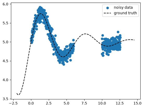
Now we generate 10x more points as in the ExactGP case, still the inference
(calculate posterior predictive distribution) and prediction won’t be much
slower (exact GPs scale roughly as \(N^3\)). Note that the data we use here is
still tiny (1000 points is easy even for exact GPs), so the method’s
usefulness cannot be fully exploited with our small scale example – also we
don’t even use a GPU yet :).
def ground_truth(x, const):
    return torch.sin(x) * torch.exp(-0.2 * x) + const


def generate_data(x, gaps=[[1, 3]], const=None, noise_std=None):
    noise_dist = torch.distributions.Normal(loc=0, scale=noise_std)
    y = ground_truth(x, const=const) + noise_dist.sample(
        sample_shape=(len(x),)
    )
    msk = torch.tensor([True] * len(x))
    if gaps is not None:
        for g in gaps:
            msk = msk & ~((x > g[0]) & (x < g[1]))
    return x[msk], y[msk], y


const = 5.0
noise_std = 0.1
x = torch.linspace(0, 4 * math.pi, 1000)
X_train, y_train, y_gt_train = generate_data(
    x, gaps=[[6, 10]], const=const, noise_std=noise_std
)
X_pred = torch.linspace(
    X_train[0] - 2, X_train[-1] + 2, 200, requires_grad=False
)
y_gt_pred = ground_truth(X_pred, const=const)

print(f"{X_train.shape=}")
print(f"{y_train.shape=}")
print(f"{X_pred.shape=}")

fig, ax = plt.subplots()
ax.scatter(X_train, y_train, marker="o", color="tab:blue", label="noisy data")
ax.plot(X_pred, y_gt_pred, ls="--", color="k", label="ground truth")
ax.legend()

if is_interactive():
    plt.show()
X_train.shape=torch.Size([682])
y_train.shape=torch.Size([682])
X_pred.shape=torch.Size([200])
Define GP model#
The model follows this example based on Hensman et al., “Scalable Variational Gaussian Process Classification”, 2015. The model is “sparse” since it works with a set of inducing points \((\ma Z, \ve u), \ve u=f(\ma Z)\) with \(f\) the unknown ground truth function. This inducing points data set is much smaller than the train data \((\ma X, \ve y)\). At prediction time, the model will use only this small data set instead of the full training data set as vanilla GPs would. This makes prediction scale to large data sets. See also the GPJax docs for a nice introduction.
We have the same hyper parameters as before
\(\ell\) =
model.covar_module.base_kernel.lengthscale\(\sigma_n^2\) =
likelihood.noise_covar.noise\(s\) =
model.covar_module.outputscale\(m(\ve x) = c\) =
model.mean_module.constant
plus additional ones, introduced by the approximations used (more details below):
the learnable inducing points \(\ma Z\) for the variational distribution \(q_{\ve\psi}(\ve u)\)
learnable parameters \(\ve m_u\) and \(\ma L\) of the variational distribution \(q_{\ve\psi}(\ve u)=\mathcal N(\ve m_u, \ma S)\): the variational mean \(\ve m_u\) and covariance \(\ma S\) in form a lower triangular matrix \(\ma L\) such that \(\ma S=\ma L\,\ma L^\top\) (Cholesky decomposition of \(\ma S\), so we store only \(\ma L\))
In the code below:
\(\ma Z\) =
model.variational_strategy.inducing_points\(\ve m_u\) =
model.variational_strategy._variational_distribution.variational_mean\(\ma L\) =
model.variational_strategy._variational_distribution.chol_variational_covar
class ApproxGPModel(gpytorch.models.ApproximateGP):
    def __init__(self, Z):
        # Approximate inducing value posterior q(u), u = f(Z), Z = inducing
        # points (subset of X_train)
        variational_distribution = (
            gpytorch.variational.CholeskyVariationalDistribution(Z.size(0))
        )
        # Compute q(f(X)) from q(u)
        variational_strategy = gpytorch.variational.VariationalStrategy(
            self,
            Z,
            variational_distribution,
            learn_inducing_locations=True,
        )
        super().__init__(variational_strategy)
        self.mean_module = gpytorch.means.ConstantMean()
        self.covar_module = gpytorch.kernels.ScaleKernel(
            gpytorch.kernels.RBFKernel()
        )

    def forward(self, x):
        mean_x = self.mean_module(x)
        covar_x = self.covar_module(x)
        return gpytorch.distributions.MultivariateNormal(mean_x, covar_x)


likelihood = gpytorch.likelihoods.GaussianLikelihood()
Now we initialize the model by defining optimization start values for the
inducing points \(\ma Z\). We use a 5% random sub-sample of X_train, so we
effectively reduce the data size used during prediction by a factor of 20. The
learning process (below) will find an optimal set of inducing points that
approximately represents the full dataset.
n_train = len(X_train)
ind_points_fraction = 0.05
ind_idxs = torch.randperm(n_train)[: int(n_train * ind_points_fraction)]
print(f"Number of inducing points={len(ind_idxs)}")
model = ApproxGPModel(Z=X_train[ind_idxs])
Number of inducing points=34
# Inspect the model
print(model)
ApproxGPModel(
  (variational_strategy): VariationalStrategy(
    (_variational_distribution): CholeskyVariationalDistribution()
  )
  (mean_module): ConstantMean()
  (covar_module): ScaleKernel(
    (base_kernel): RBFKernel(
      (raw_lengthscale_constraint): Positive()
    )
    (raw_outputscale_constraint): Positive()
  )
)
# Inspect the likelihood. In contrast to ExactGP, the likelihood is not part of
# the GP model instance.
print(likelihood)
GaussianLikelihood(
  (noise_covar): HomoskedasticNoise(
    (raw_noise_constraint): GreaterThan(1.000E-04)
  )
)
# Default start hyper params
print("model params:")
pprint(extract_model_params(model))
print("likelihood params:")
pprint(extract_model_params(likelihood))
model params:
{'covar_module.base_kernel.lengthscale': tensor([[0.6931]], grad_fn=<SoftplusBackward0>),
 'covar_module.outputscale': tensor(0.6931, grad_fn=<SoftplusBackward0>),
 'mean_module.constant': Parameter containing:
tensor(0., requires_grad=True),
 'variational_strategy._variational_distribution.chol_variational_covar': Parameter containing:
tensor([[1., 0., 0.,  ..., 0., 0., 0.],
        [0., 1., 0.,  ..., 0., 0., 0.],
        [0., 0., 1.,  ..., 0., 0., 0.],
        ...,
        [0., 0., 0.,  ..., 1., 0., 0.],
        [0., 0., 0.,  ..., 0., 1., 0.],
        [0., 0., 0.,  ..., 0., 0., 1.]], requires_grad=True),
 'variational_strategy._variational_distribution.variational_mean': Parameter containing:
tensor([0., 0., 0., 0., 0., 0., 0., 0., 0., 0., 0., 0., 0., 0., 0., 0., 0., 0., 0., 0., 0., 0., 0., 0.,
        0., 0., 0., 0., 0., 0., 0., 0., 0., 0.], requires_grad=True),
 'variational_strategy.inducing_points': Parameter containing:
tensor([[ 0.2264],
        [11.6229],
        [12.0129],
        [ 3.5598],
        [ 4.5787],
        [10.9437],
        [11.6858],
        [ 0.6415],
        [10.4154],
        [ 2.4152],
        [10.7298],
        [ 0.9434],
        [ 5.5976],
        [ 4.4404],
        [ 3.2328],
        [ 4.7171],
        [11.4594],
        [ 1.4843],
        [ 2.8051],
        [ 0.3774],
        [ 1.4717],
        [ 0.8176],
        [10.7047],
        [ 4.8052],
        [ 1.8743],
        [ 0.6289],
        [11.2330],
        [ 5.2706],
        [ 0.2642],
        [ 3.6731],
        [ 3.9624],
        [ 5.3586],
        [10.7173],
        [ 4.8555]], requires_grad=True)}
likelihood params:
{'noise_covar.noise': tensor([0.6932], grad_fn=<AddBackward0>)}
# Set new start hyper params (scalars only)
model.mean_module.constant = 3.0
model.covar_module.base_kernel.lengthscale = 1.0
model.covar_module.outputscale = 1.0
likelihood.noise_covar.noise = 0.3
Fit GP to data: optimize hyper params#
In contrast to ExactGP, we will approximate the exact posterior by a
distribution \(q_{\ve\zeta}\) (with parameters \(\ve\zeta\)) which uses
the inducing points. To find that distribution, we optimize the GP hyper
parameters by doing a GP-specific variational inference (VI), where we don’t
maximize the log marginal likelihood (ExactGP case), but an ELBO (“evidence
lower bound”) objective – a lower bound on the marginal likelihood (the
“evidence”). In variational inference, an ELBO objective shows up when
minimizing the KL divergence between an approximate and the true posterior.
Starting with Bayes’ rule
we obtain the optimal variational parameters \(\ve\zeta^*\) to approximate the true posterior \(p(w|y)\) with \(q_{\ve\zeta^*}(w)\) by
In our case the two distributions are the approximate “variational strategy”
which maps the inducing points \(\ve u = f(\ma Z)\) to the full data set \(\predve f = f(\ma X)\), and the true posterior \(p(\mathbf f|\mathcal D)\) over function values. We optimize with respect to
with
the parameters of the variational distribution \(q_{\ve\psi}(\ve u)\).
In addition, we perform a stochastic optimization by using a deep learning
type mini-batch loop, hence “stochastic” variational inference (SVI). The
latter speeds up the optimization since we only look at a fraction of data
per optimizer step to calculate an approximate loss gradient
(loss.backward()). Next to using inducing points to speed up prediction, this
performance improvement technique makes it possible to train with large
amounts of data.
# Train mode
model.train()
likelihood.train()

optimizer = torch.optim.Adam(
    [dict(params=model.parameters()), dict(params=likelihood.parameters())],
    lr=0.1,
)
loss_func = gpytorch.mlls.VariationalELBO(
    likelihood, model, num_data=X_train.shape[0]
)

train_dl = DataLoader(
    TensorDataset(X_train, y_train), batch_size=128, shuffle=True
)

n_iter = 50
history = defaultdict(list)
for i_iter in range(n_iter):
    for i_batch, (X_batch, y_batch) in enumerate(train_dl):
        batch_history = defaultdict(list)
        optimizer.zero_grad()
        loss = -loss_func(model(X_batch), y_batch)
        loss.backward()
        optimizer.step()
        param_dct = dict()
        param_dct.update(extract_model_params(model, try_item=True))
        param_dct.update(extract_model_params(likelihood, try_item=True))
        for p_name, p_val in param_dct.items():
            if isinstance(p_val, float):
                batch_history[p_name].append(p_val)
        batch_history["loss"].append(loss.item())
    for p_name, p_lst in batch_history.items():
        history[p_name].append(np.mean(p_lst))
    if (i_iter + 1) % 10 == 0:
        print(f"iter {i_iter + 1}/{n_iter}, {loss=:.3f}")
iter 10/50, loss=0.572
iter 20/50, loss=-0.361
iter 30/50, loss=-0.777
iter 40/50, loss=-0.880
iter 50/50, loss=-0.922
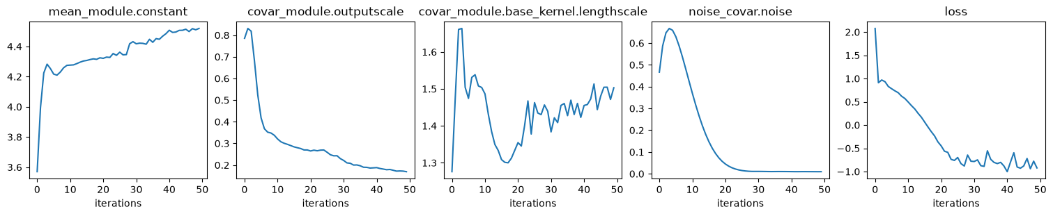
# Plot scalar hyper params and loss (ELBO) convergence
ncols = len(history)
fig, axs = plt.subplots(
    ncols=ncols, nrows=1, figsize=(ncols * 3, 3), layout="compressed"
)
with torch.no_grad():
    for ax, (p_name, p_lst) in zip(axs, history.items()):
        ax.plot(p_lst)
        ax.set_title(p_name)
        ax.set_xlabel("iterations")

if is_interactive():
    plt.show()
# Values of optimized hyper params
print("model params:")
pprint(extract_model_params(model))
print("likelihood params:")
pprint(extract_model_params(likelihood))
model params:
{'covar_module.base_kernel.lengthscale': tensor([[1.5031]], grad_fn=<SoftplusBackward0>),
 'covar_module.outputscale': tensor(0.1694, grad_fn=<SoftplusBackward0>),
 'mean_module.constant': Parameter containing:
tensor(4.5193, requires_grad=True),
 'variational_strategy._variational_distribution.chol_variational_covar': Parameter containing:
tensor([[ 3.7566e-02,  0.0000e+00,  0.0000e+00,  ...,  0.0000e+00,
          0.0000e+00,  0.0000e+00],
        [ 3.3445e-04,  1.9769e-02,  0.0000e+00,  ...,  0.0000e+00,
          0.0000e+00,  0.0000e+00],
        [ 7.6284e-04, -3.6652e-02,  4.7425e-02,  ...,  0.0000e+00,
          0.0000e+00,  0.0000e+00],
        ...,
        [ 7.1240e-03, -2.0032e-04, -2.7415e-03,  ...,  9.9990e-01,
          0.0000e+00,  0.0000e+00],
        [ 2.9062e-03,  6.7112e-03, -1.7664e-03,  ...,  8.0390e-04,
          9.9921e-01,  0.0000e+00],
        [ 3.8467e-03, -7.7030e-04,  2.5943e-03,  ..., -2.3468e-04,
         -2.6701e-04,  9.9984e-01]], requires_grad=True),
 'variational_strategy._variational_distribution.variational_mean': Parameter containing:
tensor([ 1.6601e+00,  9.5832e-01,  4.9854e-01,  6.2027e-01,  7.9282e-02,
         7.9551e-01,  4.2044e-02,  8.2212e-01,  1.1970e-01,  2.2252e+00,
         1.7954e-01,  1.7490e+00,  1.0354e+00,  9.6497e-03, -8.0405e-02,
        -2.9831e-02, -8.9635e-02,  9.7873e-02,  7.2295e-03, -3.4739e-02,
        -9.1347e-04,  7.3946e-02, -2.6763e-01, -1.0210e-02, -2.4873e-02,
         5.6441e-02,  8.7831e-02,  3.9166e-02,  9.0045e-03,  4.1844e-02,
         1.1125e-02,  1.1019e-02,  3.6794e-02,  3.2019e-02],
       requires_grad=True),
 'variational_strategy.inducing_points': Parameter containing:
tensor([[ 2.2137e-01],
        [ 1.1420e+01],
        [ 1.2184e+01],
        [ 3.4854e+00],
        [ 5.1341e+00],
        [ 1.0199e+01],
        [ 1.2885e+01],
        [-3.9406e+00],
        [ 1.1780e+01],
        [ 2.5042e+00],
        [ 9.5413e+00],
        [ 6.4558e-01],
        [ 6.3554e+00],
        [ 4.1642e+00],
        [ 2.9059e+00],
        [ 4.7003e+00],
        [ 1.2412e+01],
        [-8.1250e-01],
        [ 4.0233e+00],
        [ 3.5713e-01],
        [ 3.3160e+00],
        [ 1.4693e+00],
        [ 1.1050e+01],
        [ 4.1033e+00],
        [ 2.1501e+00],
        [ 1.3723e+00],
        [ 9.9115e+00],
        [ 4.6978e+00],
        [ 8.7772e-03],
        [ 3.4579e+00],
        [ 2.9419e+00],
        [ 4.1294e+00],
        [ 9.7329e+00],
        [ 3.5045e+00]], requires_grad=True)}
likelihood params:
{'noise_covar.noise': tensor([0.0098], grad_fn=<AddBackward0>)}
Run prediction#
# Evaluation (predictive posterior) mode
model.eval()
likelihood.eval()
with torch.no_grad():
M = 10
post_pred_f = model(X_pred)
post_pred_y = likelihood(model(X_pred))
fig, axs = plt.subplots(ncols=2, figsize=(14, 5), sharex=True, sharey=True)
fig_sigmas, ax_sigmas = plt.subplots()
for ii, (ax, post_pred, name, title) in enumerate(
zip(
axs,
[post_pred_f, post_pred_y],
["f", "y"],
["epistemic uncertainty", "total uncertainty"],
)
):
yf_mean = post_pred.mean
yf_samples = post_pred.sample(sample_shape=torch.Size((M,)))
yf_std = post_pred.stddev
lower = yf_mean - 2 * yf_std
upper = yf_mean + 2 * yf_std
y_min = y_train.min()
y_max = y_train.max()
y_span = y_max - y_min
ax.scatter(
X_train.numpy(),
y_train.numpy(),
marker="o",
label="data",
color="tab:gray",
alpha=0.2,
)
ax.plot(
X_pred.numpy(),
yf_mean.numpy(),
label="mean",
color="tab:red",
lw=2,
)
ax.plot(
X_pred.numpy(),
y_gt_pred.numpy(),
label="ground truth",
color="k",
lw=2,
ls="--",
)
ax.fill_between(
X_pred.numpy(),
lower.numpy(),
upper.numpy(),
label="confidence",
color="tab:orange",
alpha=0.3,
)
ax.set_title(f"confidence = {title}")
if name == "f":
sigma_label = r"epistemic: $\pm 2\sqrt{\mathrm{diag}(\Sigma_*)}$"
zorder = 1
else:
sigma_label = (
r"total: $\pm 2\sqrt{\mathrm{diag}(\Sigma_* + \sigma_n^2\,I)}$"
)
zorder = 0
ax.set_ylim([y_min - 0.3 * y_span, y_max + 0.3 * y_span])
ax.scatter(
model.variational_strategy.inducing_points.numpy(),
[y_min] * len(model.variational_strategy.inducing_points),
marker="o",
label="inducing points",
color="tab:blue",
)
if ii == 1:
ax.legend()
ax_sigmas.fill_between(
X_pred.numpy(),
lower.numpy(),
upper.numpy(),
label=sigma_label,
color="tab:orange" if name == "f" else "tab:blue",
alpha=0.5,
zorder=zorder,
)
plot_samples(ax, X_pred, yf_samples, label="posterior pred. samples")
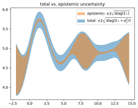
ax_sigmas.set_title("total vs. epistemic uncertainty")
ax_sigmas.legend()
if is_interactive():
plt.show()
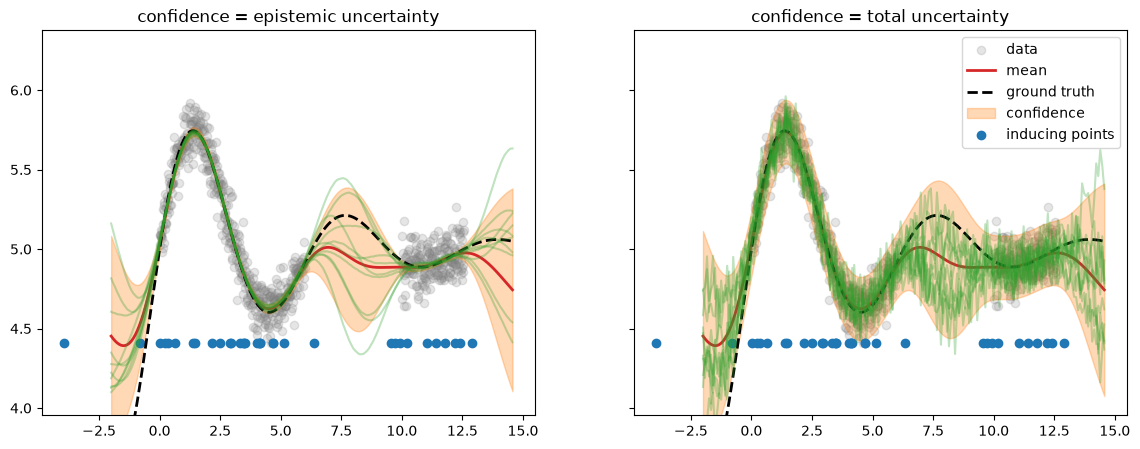
We get a result which is very similar to the ExactGP case. Note that the
inducing points \(\ma Z\) (initialized randomly uniform along \(x\)) are now
concentrated in the regions of high data density and not in the
out-of-distribution “gap” in the middle.
Let’s check the learned noise#
# Target noise to learn
print("data noise:", noise_std)

# The two below must be the same
print(
    "learned noise:",
    (post_pred_y.stddev**2 - post_pred_f.stddev**2).mean().sqrt().item(),
)
print(
    "learned noise:",
    np.sqrt(
        extract_model_params(likelihood, try_item=True)["noise_covar.noise"]
    ),
)
data noise: 0.1
learned noise: 0.09910244654748243
learned noise: 0.09910244654748243
# When running as script
if not is_interactive():
    plt.show()