1D exact GP regression

In this notebook, we explore the material presented in the slides with code, using the gpytorch library. We cover exact GP inference and hyper parameter optimization using the marginal likelihood.

The notebook is inspired by the Exact GP Regression example from the gpytorch docs.

Notation

\(\newcommand{\ve}[1]{\mathit{\boldsymbol{#1}}}\) \(\newcommand{\ma}[1]{\mathbf{#1}}\) \(\newcommand{\pred}[1]{\rm{#1}}\) \(\newcommand{\predve}[1]{\mathbf{#1}}\) \(\newcommand{\test}[1]{#1_*}\) \(\newcommand{\testtest}[1]{#1_{**}}\) \(\DeclareMathOperator{\diag}{diag}\) \(\DeclareMathOperator{\cov}{cov}\)

Vector \(\ve a\in\mathbb R^n\) or \(\mathbb R^{n\times 1}\), so “column” vector. Matrix \(\ma A\in\mathbb R^{n\times m}\). Design matrix with input vectors \(\ve x_i\in\mathbb R^D\): \(\ma X = [\ldots, \ve x_i, \ldots]^\top \in\mathbb R^{N\times D}\).

We use 1D data, so in fact \(\ma X \in\mathbb R^{N\times 1}\) is a vector, but we still denote the collection of all \(\ve x_i = x_i\in\mathbb R\) points with \(\ma X\) to keep the notation consistent with the slides.

Imports, helpers, setup

##%matplotlib notebook
##%matplotlib widget
%matplotlib inline

import math
from collections import defaultdict
from pprint import pprint

import torch
import gpytorch
from matplotlib import pyplot as plt
from matplotlib import is_interactive
import numpy as np

from utils import extract_model_params, plot_samples


# Default float32 results in slightly noisy prior samples. Less so with
# float64. We get a warning with both
#   .../lib/python3.11/site-packages/linear_operator/utils/cholesky.py:40:
#       NumericalWarning: A not p.d., added jitter of 1.0e-08 to the diagonal
# but the noise is smaller w/ float64. Reason must be that the `sample()`
# method [1] calls `rsample()` [2] which performs a Cholesky decomposition of
# the covariance matrix. The default in
# np.random.default_rng().multivariate_normal() is method="svd", which is
# slower but seemingly a bit more stable.
#
# [1] https://docs.gpytorch.ai/en/stable/distributions.html#gpytorch.distributions.MultivariateNormal.sample
# [2] https://docs.gpytorch.ai/en/stable/distributions.html#gpytorch.distributions.MultivariateNormal.rsample
torch.set_default_dtype(torch.float64)

torch.manual_seed(123)

<torch._C.Generator at 0x7fd41a543cb0>

Generate toy 1D data

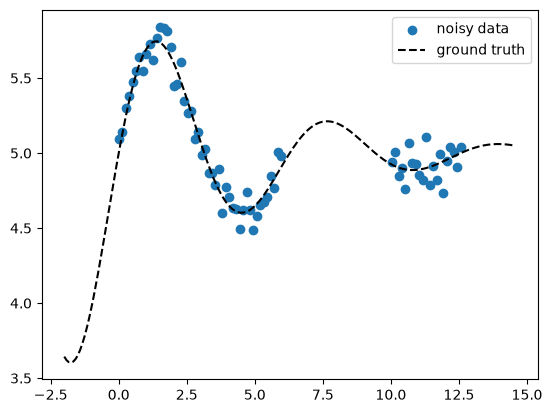
Here we generate noisy 1D data \(\ma X\) = X_train, \(\ve y\) = y_train as well as an extended x-axis \(\test{\ma X}\) = X_pred which we use later for prediction also outside of the data range (extrapolation). The data has a constant offset const which we use to test learning a GP mean function \(m(\ve x)\). We create a gap in the data to show how the model uncertainty will behave there.

def ground_truth(x, const):
    return torch.sin(x) * torch.exp(-0.2 * x) + const


def generate_data(x, gaps=[[1, 3]], const=None, noise_std=None):
    noise_dist = torch.distributions.Normal(loc=0, scale=noise_std)
    y = ground_truth(x, const=const) + noise_dist.sample(
        sample_shape=(len(x),)
    )
    msk = torch.tensor([True] * len(x))
    if gaps is not None:
        for g in gaps:
            msk = msk & ~((x > g[0]) & (x < g[1]))
    return x[msk], y[msk], y


const = 5.0
noise_std = 0.1
x = torch.linspace(0, 4 * math.pi, 100)
X_train, y_train, y_gt_train = generate_data(
    x, gaps=[[6, 10]], const=const, noise_std=noise_std
)
X_pred = torch.linspace(
    X_train[0] - 2, X_train[-1] + 2, 200, requires_grad=False
)
y_gt_pred = ground_truth(X_pred, const=const)

print(f"{X_train.shape=}")
print(f"{y_train.shape=}")
print(f"{X_pred.shape=}")

fig, ax = plt.subplots()
ax.scatter(X_train, y_train, marker="o", color="tab:blue", label="noisy data")
ax.plot(X_pred, y_gt_pred, ls="--", color="k", label="ground truth")
ax.legend()

if is_interactive():
    plt.show()

X_train.shape=torch.Size([69])
y_train.shape=torch.Size([69])
X_pred.shape=torch.Size([200])

Define GP model

We define the simplest possible textbook GP model using a Gaussian likelihood. The kernel is the squared exponential kernel with a scaling factor.

\[\kappa(\ve x_i, \ve x_j) = s\,\exp\left(-\frac{\lVert\ve x_i - \ve x_j\rVert_2^2}{2\,\ell^2}\right)\]

This makes two hyper params, namely the length scale \(\ell\) and the scaling \(s\). The latter is implemented by wrapping the RBFKernel with ScaleKernel.

In addition, we define a constant mean via ConstantMean. Finally we have the likelihood variance \(\sigma_n^2\). So in total we have 4 hyper params.

• \(\ell\) = model.covar_module.base_kernel.lengthscale

• \(\sigma_n^2\) = model.likelihood.noise_covar.noise

• \(s\) = model.covar_module.outputscale

• \(m(\ve x) = c\) = model.mean_module.constant

class ExactGPModel(gpytorch.models.ExactGP):
    """API:

    model.forward()             prior                   f_pred
    model()                     posterior               f_pred

    likelihood(model.forward()) prior with noise        y_pred
    likelihood(model())         posterior with noise    y_pred
    """

    def __init__(self, X_train, y_train, likelihood):
        super().__init__(X_train, y_train, likelihood)
        self.mean_module = gpytorch.means.ConstantMean()
        self.covar_module = gpytorch.kernels.ScaleKernel(
            gpytorch.kernels.RBFKernel()
        )

    def forward(self, x):
        """The prior, defined in terms of the mean and covariance function."""
        mean_x = self.mean_module(x)
        covar_x = self.covar_module(x)
        return gpytorch.distributions.MultivariateNormal(mean_x, covar_x)


likelihood = gpytorch.likelihoods.GaussianLikelihood()
model = ExactGPModel(X_train, y_train, likelihood)

# Inspect the model
print(model)

ExactGPModel(
  (likelihood): GaussianLikelihood(
    (noise_covar): HomoskedasticNoise(
      (raw_noise_constraint): GreaterThan(1.000E-04)
    )
  )
  (mean_module): ConstantMean()
  (covar_module): ScaleKernel(
    (base_kernel): RBFKernel(
      (raw_lengthscale_constraint): Positive()
    )
    (raw_outputscale_constraint): Positive()
  )
)

# Default start hyper params
pprint(extract_model_params(model))

{'covar_module.base_kernel.lengthscale': tensor([[0.6931]], grad_fn=<SoftplusBackward0>),
 'covar_module.outputscale': tensor(0.6931, grad_fn=<SoftplusBackward0>),
 'likelihood.noise_covar.noise': tensor([0.6932], grad_fn=<AddBackward0>),
 'mean_module.constant': Parameter containing:
tensor(0., requires_grad=True)}

# Set new start hyper params
model.mean_module.constant = 3.0
model.covar_module.base_kernel.lengthscale = 1.0
model.covar_module.outputscale = 1.0
model.likelihood.noise_covar.noise = 1e-3

pprint(extract_model_params(model))

{'covar_module.base_kernel.lengthscale': tensor([[1.]], grad_fn=<SoftplusBackward0>),
 'covar_module.outputscale': tensor(1., grad_fn=<SoftplusBackward0>),
 'likelihood.noise_covar.noise': tensor([0.0010], grad_fn=<AddBackward0>),
 'mean_module.constant': Parameter containing:
tensor(3., requires_grad=True)}

Sample from the GP prior

We sample a number of functions \(f_m, m=1,\ldots,M\) from the GP prior and evaluate them at all \(\test{\ma X}\) = X_pred points, of which we have \(\test{N}=200\). So we effectively generate samples from pri_f = \(p(\test{\predve f}|\test{\ma X}) = \mathcal N(\ve c, \testtest{\ma K})\). Each sampled vector \(\test{\predve f}\in\mathbb R^{\test{N}}\) represents a sampled function \(f_m\) evaluated at the \(\test{N}=200\) points in \(\test{\ma X}\). The covariance (kernel) matrix is \(\testtest{\ma K}\in\mathbb R^{\test{N}\times \test{N}}\) with \((\testtest{\ma K})_{ij}=\cov[f_m(\ve x_i), f_m(\ve x_j)]\). Its diagonal \(\diag\testtest{\ma K}\) = f_std**2 represents the variance at each point on the \(x\)-axis. This is what we plot as “confidence band” f_mean \(\pm\) 2 * f_std. The off-diagonal elements represent the correlation between different points along the \(x\)-axis.

model.eval()
likelihood.eval()

with torch.no_grad():
    # Prior
    M = 10
    pri_f = model.forward(X_pred)
    f_mean = pri_f.mean
    f_std = pri_f.stddev
    f_samples = pri_f.sample(sample_shape=torch.Size((M,)))
    print(f"{pri_f=}")
    print(f"{pri_f.mean.shape=}")
    print(f"{pri_f.covariance_matrix.shape=}")
    print(f"{f_samples.shape=}")
    fig, ax = plt.subplots()
    ax.plot(X_pred, f_mean, color="tab:red", label="mean", lw=2)
    plot_samples(ax, X_pred, f_samples, label="prior samples")
    ax.fill_between(
        X_pred,
        f_mean - 2 * f_std,
        f_mean + 2 * f_std,
        color="tab:orange",
        alpha=0.2,
        label="confidence",
    )
    ax.legend()

if is_interactive():
    plt.show()

pri_f=MultivariateNormal(loc: torch.Size([200]))
pri_f.mean.shape=torch.Size([200])
pri_f.covariance_matrix.shape=torch.Size([200, 200])
f_samples.shape=torch.Size([10, 200])

/opt/hostedtoolcache/Python/3.13.13/x64/lib/python3.13/site-packages/linear_operator/utils/cholesky.py:41: NumericalWarning: A not p.d., added jitter of 1.0e-08 to the diagonal
  warnings.warn(

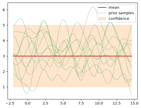
Let’s investigate the samples more closely. First we note that the samples fluctuate around the mean model.mean_module.constant we defined above. A constant mean \(\ve m(\test{\ma X}) = \ve c\) does not mean that each sampled vector \(\test{\predve f}\)’s mean is equal to \(c\). Instead, we have that at each \(\ve x_i\), the mean of all sampled functions is the same, so \(\frac{1}{M}\sum_{j=1}^M f_m(\ve x_i) \approx c\) and for \(M\rightarrow\infty\) it will be exactly \(c\).

Let’s look at the first 20 \(x\) points from \(M=10\) samples.

print(f"{f_samples.shape=}")
print(f"{f_samples.mean(axis=0)[:20]=}")
print(f"{f_samples.mean(axis=0).mean()=}")
print(f"{f_samples.mean(axis=0).std()=}")

f_samples.shape=torch.Size([10, 200])
f_samples.mean(axis=0)[:20]=tensor([3.2870, 3.2644, 3.2399, 3.2143, 3.1882, 3.1621, 3.1368, 3.1128, 3.0905,
        3.0703, 3.0522, 3.0365, 3.0230, 3.0114, 3.0016, 2.9931, 2.9856, 2.9788,
        2.9723, 2.9658])
f_samples.mean(axis=0).mean()=tensor(3.2061)
f_samples.mean(axis=0).std()=tensor(0.2459)

Take more samples, the means should get closer to \(c=3\).

f_samples = pri_f.sample(sample_shape=torch.Size((M * 200,)))
print(f"{f_samples.shape=}")
print(f"{f_samples.mean(axis=0)[:20]=}")
print(f"{f_samples.mean(axis=0).mean()=}")
print(f"{f_samples.mean(axis=0).std()=}")

f_samples.shape=torch.Size([2000, 200])
f_samples.mean(axis=0)[:20]=tensor([2.9535, 2.9550, 2.9565, 2.9580, 2.9594, 2.9609, 2.9624, 2.9639, 2.9655,
        2.9672, 2.9691, 2.9711, 2.9733, 2.9756, 2.9782, 2.9810, 2.9840, 2.9872,
        2.9904, 2.9937])
f_samples.mean(axis=0).mean()=tensor(2.9894)
f_samples.mean(axis=0).std()=tensor(0.0158)

GP posterior predictive distribution with fixed hyper params

Now we calculate the posterior predictive distribution \(p(\test{\predve f}|\test{\ma X}, \ma X, \ve y) = \mathcal N(\test{\ve\mu}, \test{\ma\Sigma})\), i.e. we condition on the train data (Bayesian inference).

We use the fixed hyper param values defined above. In particular, since \(\sigma_n^2\) = model.likelihood.noise_covar.noise is > 0, we have a regression setting – the GP’s mean doesn’t interpolate all points.

# Evaluation (predictive posterior) mode
model.eval()
likelihood.eval()

with torch.no_grad():
    M = 10
    post_pred_f = model(X_pred)

    fig, ax = plt.subplots()
    f_mean = post_pred_f.mean
    f_samples = post_pred_f.sample(sample_shape=torch.Size((M,)))
    f_std = post_pred_f.stddev
    lower = f_mean - 2 * f_std
    upper = f_mean + 2 * f_std
    ax.plot(
        X_train.numpy(),
        y_train.numpy(),
        "o",
        label="data",
        color="tab:blue",
    )
    ax.plot(
        X_pred.numpy(),
        f_mean.numpy(),
        label="mean",
        color="tab:red",
        lw=2,
    )
    ax.plot(
        X_pred.numpy(),
        y_gt_pred.numpy(),
        label="ground truth",
        color="k",
        lw=2,
        ls="--",
    )
    ax.fill_between(
        X_pred.numpy(),
        lower.numpy(),
        upper.numpy(),
        label="confidence",
        color="tab:orange",
        alpha=0.3,
    )
    y_min = y_train.min()
    y_max = y_train.max()
    y_span = y_max - y_min
    ax.set_ylim([y_min - 0.3 * y_span, y_max + 0.3 * y_span])
    plot_samples(ax, X_pred, f_samples, label="posterior pred. samples")
    ax.legend()

if is_interactive():
    plt.show()

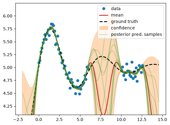
We observe that all sampled functions (green) and the mean (red) tend towards the low fixed mean function \(m(\ve x)=c\) at 3.0 in the absence of data, while the actual data mean is const = 5 from above (data generation). Also the other hyper params (\(\ell\), \(\sigma_n^2\), \(s\)) are just guesses. Now we will calculate their actual value by minimizing the negative log marginal likelihood.

Fit GP to data: optimize hyper params

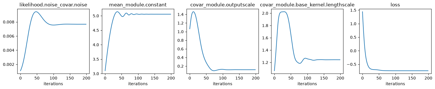
In each step of the optimizer, we condition on the training data (e.g. do Bayesian inference) to calculate the posterior predictive distribution for the current values of the hyper params. We iterate until the negative log marginal likelihood is converged.

We use a simplistic PyTorch-style hand written train loop without convergence control, so make sure to use enough n_iter and eyeball-check that the loss is converged :-)

# Train mode
model.train()
likelihood.train()

optimizer = torch.optim.Adam(model.parameters(), lr=0.1)
loss_func = gpytorch.mlls.ExactMarginalLogLikelihood(likelihood, model)

n_iter = 200
history = defaultdict(list)
for ii in range(n_iter):
    optimizer.zero_grad()
    loss = -loss_func(model(X_train), y_train)
    loss.backward()
    optimizer.step()
    if (ii + 1) % 10 == 0:
        print(f"iter {ii + 1}/{n_iter}, {loss=:.3f}")
    for p_name, p_val in extract_model_params(model, try_item=True).items():
        history[p_name].append(p_val)
    history["loss"].append(loss.item())

iter 10/200, loss=-0.133
iter 20/200, loss=-0.603
iter 30/200, loss=-0.689
iter 40/200, loss=-0.700
iter 50/200, loss=-0.712
iter 60/200, loss=-0.730
iter 70/200, loss=-0.737
iter 80/200, loss=-0.738
iter 90/200, loss=-0.739
iter 100/200, loss=-0.739
iter 110/200, loss=-0.739
iter 120/200, loss=-0.739
iter 130/200, loss=-0.739
iter 140/200, loss=-0.739
iter 150/200, loss=-0.739
iter 160/200, loss=-0.739
iter 170/200, loss=-0.739
iter 180/200, loss=-0.739
iter 190/200, loss=-0.739
iter 200/200, loss=-0.739

# Plot hyper params and loss (negative log marginal likelihood) convergence
ncols = len(history)
fig, axs = plt.subplots(
    ncols=ncols, nrows=1, figsize=(ncols * 3, 3), layout="compressed"
)
with torch.no_grad():
    for ax, (p_name, p_lst) in zip(axs, history.items()):
        ax.plot(p_lst)
        ax.set_title(p_name)
        ax.set_xlabel("iterations")

if is_interactive():
    plt.show()

# Values of optimized hyper params
pprint(extract_model_params(model))

{'covar_module.base_kernel.lengthscale': tensor([[1.2430]], grad_fn=<SoftplusBackward0>),
 'covar_module.outputscale': tensor(0.1167, grad_fn=<SoftplusBackward0>),
 'likelihood.noise_covar.noise': tensor([0.0077], grad_fn=<AddBackward0>),
 'mean_module.constant': Parameter containing:
tensor(5.0548, requires_grad=True)}

We see that all hyper params converge. In particular, note that the constant mean \(m(\ve x)=c\) converges to the const value in generate_data().

Run prediction

We run prediction with two variants of the posterior predictive distribution: using either only the epistemic uncertainty or using the total uncertainty.

• epistemic: \(p(\test{\predve f}|\test{\ma X}, \ma X, \ve y) = \mathcal N(\test{\ve\mu}, \test{\ma\Sigma})\) = post_pred_f with \(\test{\ma\Sigma} = \testtest{\ma K} - \test{\ma K}\,(\ma K+\sigma_n^2\,\ma I)^{-1}\,\test{\ma K}^\top\)

• total: \(p(\test{\ve y}|\test{\ma X}, \ma X, \ve y) = \mathcal N(\test{\ve\mu}, \test{\ma\Sigma} + \sigma_n^2\,\ma I_N))\) = post_pred_y

# Evaluation (predictive posterior) mode
model.eval()
likelihood.eval()

with torch.no_grad():
    M = 10
    post_pred_f = model(X_pred)
    post_pred_y = likelihood(model(X_pred))

    fig, axs = plt.subplots(ncols=2, figsize=(14, 5), sharex=True, sharey=True)
    fig_sigmas, ax_sigmas = plt.subplots()
    for ii, (ax, post_pred, name, title) in enumerate(
        zip(
            axs,
            [post_pred_f, post_pred_y],
            ["f", "y"],
            ["epistemic uncertainty", "total uncertainty"],
        )
    ):
        yf_mean = post_pred.mean
        yf_samples = post_pred.sample(sample_shape=torch.Size((M,)))

        yf_std = post_pred.stddev
        lower = yf_mean - 2 * yf_std
        upper = yf_mean + 2 * yf_std
        ax.plot(
            X_train.numpy(),
            y_train.numpy(),
            "o",
            label="data",
            color="tab:blue",
        )
        ax.plot(
            X_pred.numpy(),
            yf_mean.numpy(),
            label="mean",
            color="tab:red",
            lw=2,
        )
        ax.plot(
            X_pred.numpy(),
            y_gt_pred.numpy(),
            label="ground truth",
            color="k",
            lw=2,
            ls="--",
        )
        ax.fill_between(
            X_pred.numpy(),
            lower.numpy(),
            upper.numpy(),
            label="confidence",
            color="tab:orange",
            alpha=0.3,
        )
        ax.set_title(f"confidence = {title}")
        if name == "f":
            sigma_label = r"epistemic: $\pm 2\sqrt{\mathrm{diag}(\Sigma_*)}$"
            zorder = 1
        else:
            sigma_label = (
                r"total: $\pm 2\sqrt{\mathrm{diag}(\Sigma_* + \sigma_n^2\,I)}$"
            )
            zorder = 0
        ax_sigmas.fill_between(
            X_pred.numpy(),
            lower.numpy(),
            upper.numpy(),
            label=sigma_label,
            color="tab:orange" if name == "f" else "tab:blue",
            alpha=0.5,
            zorder=zorder,
        )
        y_min = y_train.min()
        y_max = y_train.max()
        y_span = y_max - y_min
        ax.set_ylim([y_min - 0.3 * y_span, y_max + 0.3 * y_span])
        plot_samples(ax, X_pred, yf_samples, label="posterior pred. samples")
        if ii == 1:
            ax.legend()
    ax_sigmas.set_title("total vs. epistemic uncertainty")
    ax_sigmas.legend()

if is_interactive():
    plt.show()

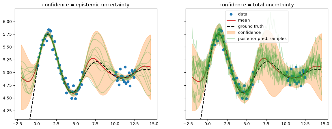
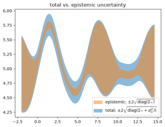
We find that \(\test{\ma\Sigma}\) reflects behavior we would like to see from epistemic uncertainty – it is high when we have no data (out-of-distribution). But this alone isn’t the whole story. We need to add the estimated likelihood variance \(\sigma_n^2\) in order for the confidence band to cover the data – this turns the estimated total uncertainty into a calibrated uncertainty.

Let’s check the learned noise

We compare the target data noise (noise_std) to the learned GP noise, in the form of the likelihood standard deviation \(\sigma_n\). The latter is equal to the \(\sqrt{\cdot}\) of likelihood.noise_covar.noise and can also be calculated via \(\sqrt{\diag(\test{\ma\Sigma} + \sigma_n^2\,\ma I_N) - \diag(\test{\ma\Sigma}})\).

# Target noise to learn
print("data noise:", noise_std)

# The two below must be the same
print(
    "learned noise:",
    (post_pred_y.stddev**2 - post_pred_f.stddev**2).mean().sqrt().item(),
)
print(
    "learned noise:",
    np.sqrt(
        extract_model_params(model, try_item=True)[
            "likelihood.noise_covar.noise"
        ]
    ),
)

data noise: 0.1
learned noise: 0.08758186260974413
learned noise: 0.08758186260974413

# When running as script
if not is_interactive():
    plt.show()