Prior and (noisy) posterior predictions

Prior and (noisy) posterior predictions#

Show the difference between noisy and noiseless predictions by plotting. Now we generate 1\(D\) toy data \((x_i\in\mathbb R, y_i\in\mathbb R)\) and also perform a “real GP fit” by optimizing the \(\ell\) hyperparameter. However we fix \(\sigma_n^2\) to certain values to showcase the different noise cases.

Below \(\ma\Sigma\equiv\cov(\ve f_*)\) is the covariance matrix from [RW06] eq. 2.24 with \(\ma K = K(X,X)\), \(\ma K'=K(X_*, X)\) and \(\ma K''=K(X_*, X_*)\), so

\[\ma\Sigma = \ma K'' - \ma K'\,(\ma K+\sigma_n^2\,\ma I)^{-1}\,\ma K'^\top\]

Imports and helpers

Show code cell source

Hide code cell source

from functools import partial

from box import Box

import numpy as np

from sklearn.gaussian_process import GaussianProcessRegressor
from sklearn.gaussian_process.kernels import RBF, WhiteKernel
from sklearn.preprocessing import StandardScaler

import matplotlib.pyplot as plt
from matplotlib import is_interactive

from common import (
    textbook_prior,
    textbook_posterior,
    textbook_posterior_noise,
    cov2std,
    sample_y,
)

plt.rcParams["figure.autolayout"] = True
plt.rcParams["font.size"] = 18


def transform_labels(name: str):
    lmap = dict(
        noise_level=r"$\sigma_n^2$",
        length_scale=r"$\ell$",
        y_std_pn=r"$\sqrt{\mathrm{diag}(\Sigma)}$",
        y_std_p=r"$\sqrt{\mathrm{diag}(\Sigma + \sigma_n^2\,I)}$",
        y_mean=r"$\mu$",
    )
    return lmap.get(name, name)


def gt_func(x):
    """Ground truth"""
    return np.sin(x) * np.exp(-0.1 * x) + 10


def transform_1d(scaler: StandardScaler, x):
    assert x.ndim == 1
    return scaler.transform(x.reshape(-1, 1))[:, 0]


def calc_gp(
    *,
    pri_post: bool,
    noise_level: float,
    pred_mode: str,
    XI: np.ndarray,
    X: np.ndarray = None,
    y: np.ndarray = None,
):
    if pri_post == "pri":
        length_scale = 0.5
        gp = GaussianProcessRegressor(
            kernel=RBF(length_scale=length_scale)
            + WhiteKernel(noise_level=noise_level),
            alpha=0,
            normalize_y=False,
        )
    elif pri_post == "post":
        gp = GaussianProcessRegressor(
            kernel=RBF(length_scale_bounds=[1e-5, 10])
            + WhiteKernel(noise_level=noise_level, noise_level_bounds="fixed"),
            n_restarts_optimizer=5,
            alpha=0,
            normalize_y=False,
        )

        gp.fit(X, y)
        length_scale = gp.kernel_.k1.length_scale
        # gp.kernel_.k2.noise_level == noise_level (fixed)
    else:
        raise ValueError(f"unknown {pri_post=}")

    y_mean, y_cov = gp.predict(XI, return_cov=True)

    if pred_mode == "p":
        post_ref_func = textbook_posterior_noise
    elif pred_mode == "pn":
        post_ref_func = textbook_posterior
        y_cov -= np.eye(XI.shape[0]) * noise_level
    else:
        raise ValueError(f"unknown {pred_mode=}")

    y_std_label = transform_labels(f"y_std_{pred_mode}")
    y_std = cov2std(y_cov)

    if pri_post == "pri":
        y_mean_ref, y_std_ref, y_cov_ref = textbook_prior(
            noise_level=noise_level, length_scale=length_scale
        )(XI)
    else:
        y_mean_ref, y_std_ref, y_cov_ref = post_ref_func(
            X, y, noise_level=noise_level, length_scale=length_scale
        )(XI)

    np.testing.assert_allclose(y_mean, y_mean_ref, rtol=0, atol=1e-9)
    np.testing.assert_allclose(y_std, y_std_ref, rtol=0, atol=1e-9)
    np.testing.assert_allclose(y_cov, y_cov_ref, rtol=0, atol=1e-9)

    samples = sample_y(y_mean, y_cov, 10, random_state=123)

    if pri_post == "pri":
        if noise_level == 0:
            cov_title = r"$\Sigma=K''$"
        else:
            cov_title = r"$\Sigma=K'' + \sigma_n^2\,I$"
    else:
        if noise_level == 0:
            cov_title = r"$\Sigma=K'' - K'\,K^{-1}\,K'^\top$"
        else:
            cov_title = r"$\Sigma=K'' - K'\,(K+\sigma_n^2\,I)^{-1}\,K'^\top$"

    cov_title += "\n" + rf"$\sigma$={y_std_label}"

    return Box(
        y_mean=y_mean,
        y_cov=y_cov,
        y_std=y_std,
        samples=samples,
        cov_title=cov_title,
        length_scale=length_scale,
        noise_level=noise_level,
        y_std_label=y_std_label,
        pri_post=pri_post,
    )


def plot_gp(
    *, box: Box, ax, xi, std_color="tab:orange", x=None, y=None, set_title=True
):
    if set_title:
        ax.set_title(
            f"{transform_labels('noise_level')}={box.noise_level}   "
            f"{transform_labels('length_scale')}={box.length_scale:.5f}"
            "\n" + box.cov_title
        )

    samples_kind = "prior" if box.pri_post == "pri" else "posterior"
    for ii, yy in enumerate(box.samples.T):
        ax.plot(
            xi,
            yy,
            color="tab:gray",
            alpha=0.3,
            label=(f"{samples_kind} samples" if ii == 0 else "_"),
        )

    ax.plot(
        xi,
        box.y_mean,
        lw=3,
        color="tab:red",
        label=transform_labels("y_mean"),
    )

    if box.pri_post == "post":
        ax.plot(x, y, "o", ms=10)

    ax.fill_between(
        xi,
        box.y_mean - 2 * box.y_std,
        box.y_mean + 2 * box.y_std,
        alpha=0.1,
        color=std_color,
        label=rf"$\pm$ 2 {box.y_std_label}",
    )

Generate 1\(D\) toy data

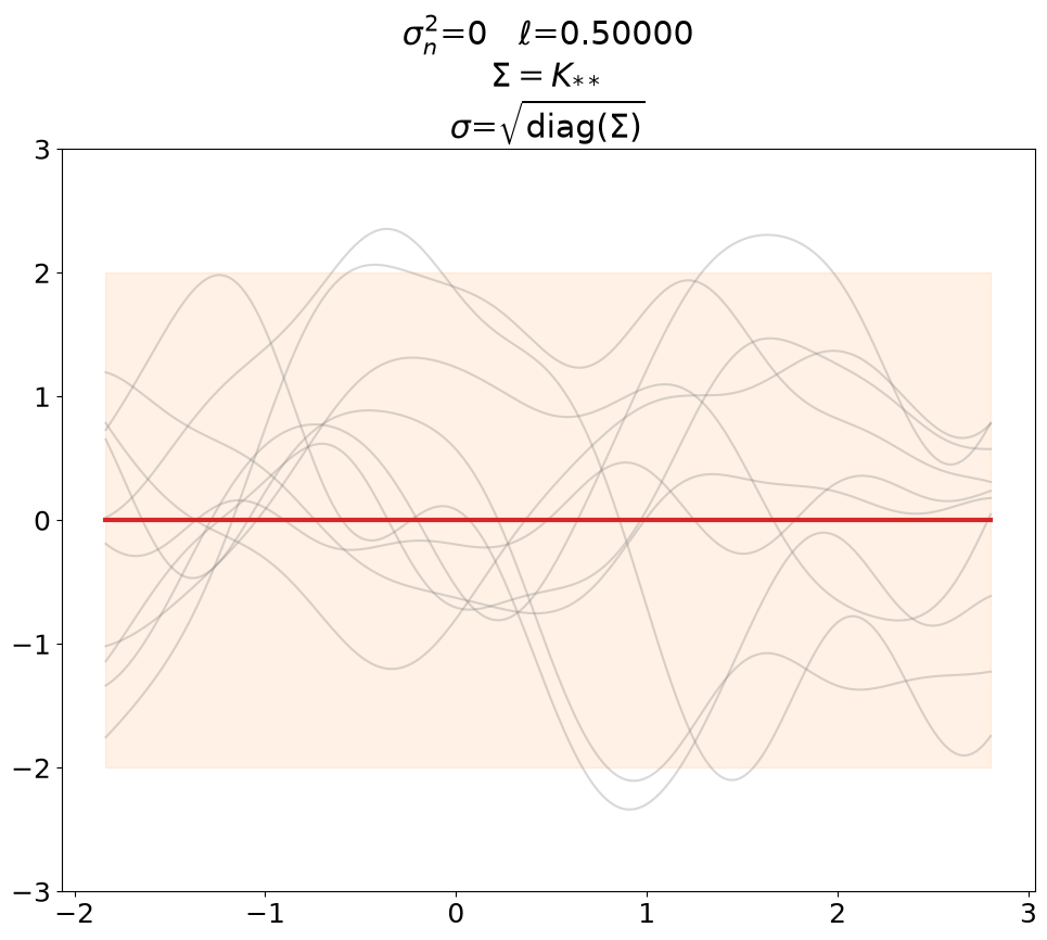
Prior, noiseless#

First we plot the prior, without noise (predict_noiseless).

This is the standard textbook case. We set \(\ell\) to some constant of our liking since its value is not defined in the absence of training data.

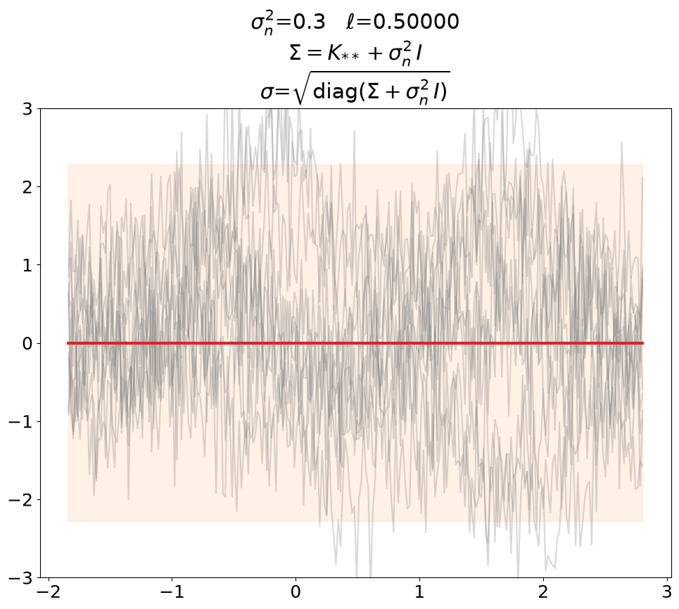
../../_images/3965b75275e641c61384f702c68f3ab47b847fc59ff3ea6f91e42b55a5400ecd.png

Prior, noisy#

Even though not super useful, we can certainly generate noisy prior samples in the predict setting when using \(\ma K'' + \sigma_n^2\,\ma I\) as prior covariance.

This is also shown in [DLvdW20] in fig. 4.

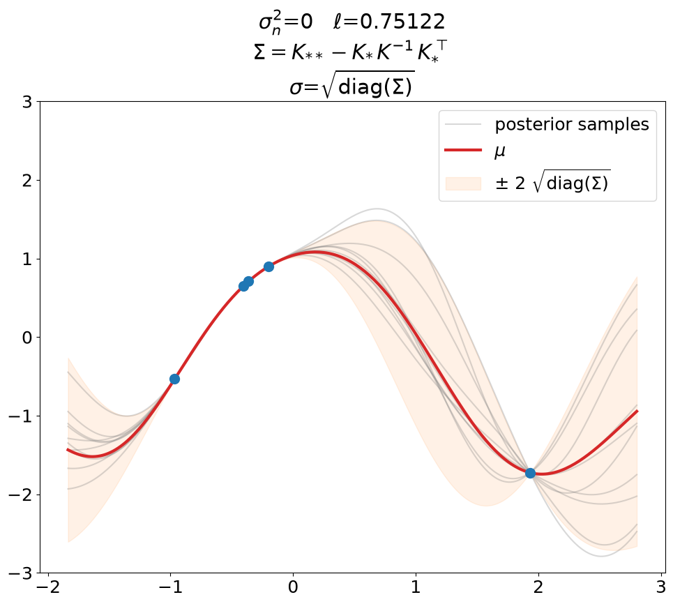
../../_images/677c26fb5f5a1cbe70d05d1070b97c188380d3fd8fbd9d808f4f343c8211a65e.png

Posterior, noiseless, interpolation#

Now the posterior.

For that, we do an \(\ell\) optimization using 1\(D\) toy data and sklearn with fixed \(\sigma_n^2\):

interpolation (\(\sigma_n = 0\))
regression (\(\sigma_n > 0\))

Interpolation (\(\sigma_n^2=0\)).

This is a plot you will see in most text books. Notice that \(\ell\) is not 0.5 as above but has been optimized (maximal LML).

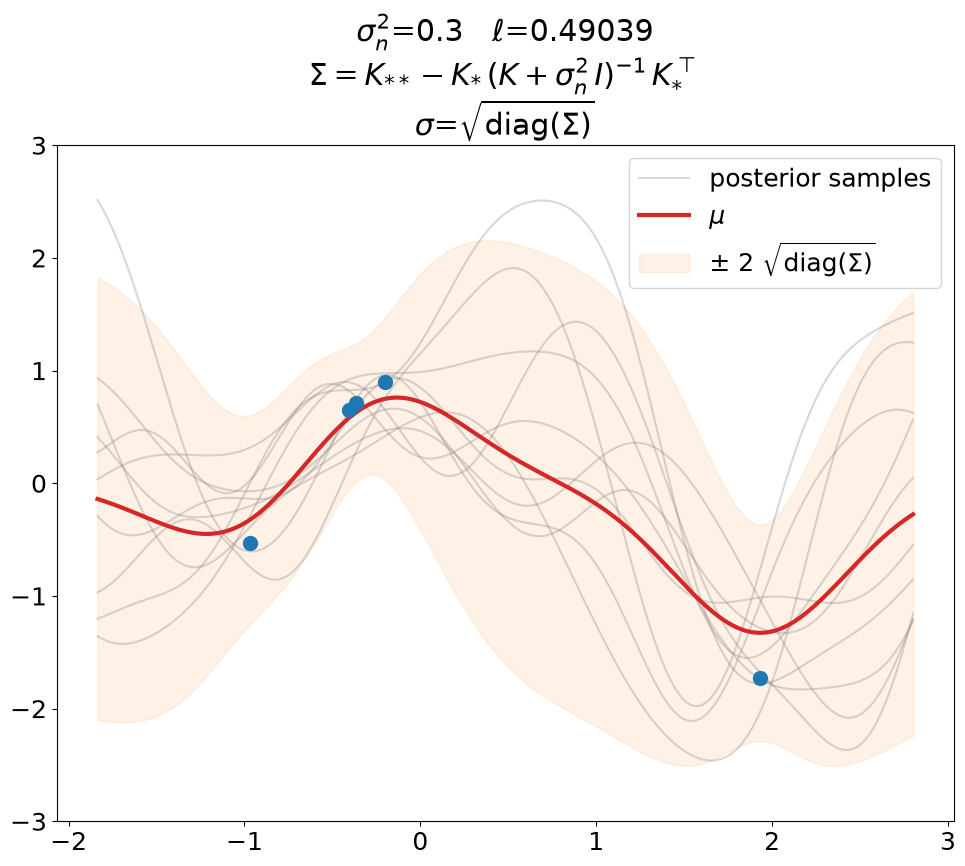
../../_images/a09e1f29588f6700aa2f18cd88ccc653fe96d3e666f1d56868a36b0bd1f9ccea.png

Posterior, noiseless, regression#

Regression (\(\sigma_n^2>0\)), predict_noiseless.

You will see a plot like this also in text books. For instance [Mur23] has this in fig. 18.7 (book version 2022-10-16). If you inspect the code that generates it (which is open source, thanks!), you find that they use tinygp in the predict_noiseless setting.

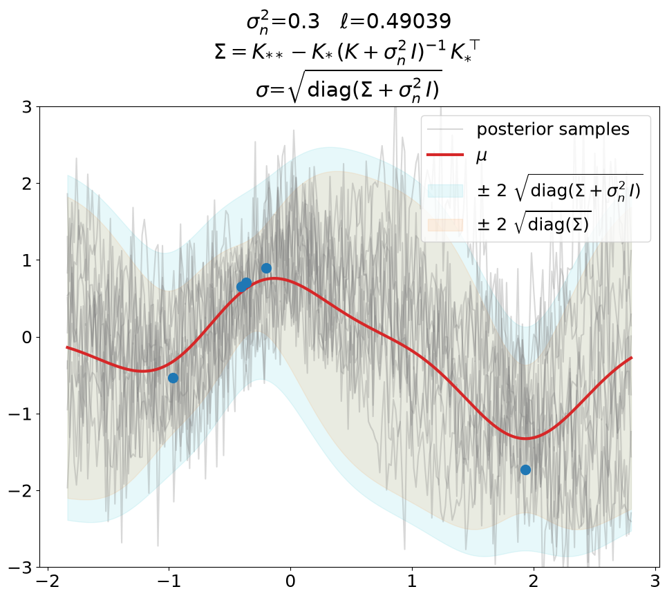
../../_images/0842ffb0d00bb461787c673cb425003ed376bb6f8dd5d8856788ded35c800560.png

Posterior, noisy, regression#

Regression (\(\sigma_n^2>0\)), predict.

This is the same as above in terms of optimized \(\ell\), \(\sigma_n^2\) value (fixed here, usually also optimized), fit weights \(\ve\alpha\) and thus predictions \(\ve\mu\).

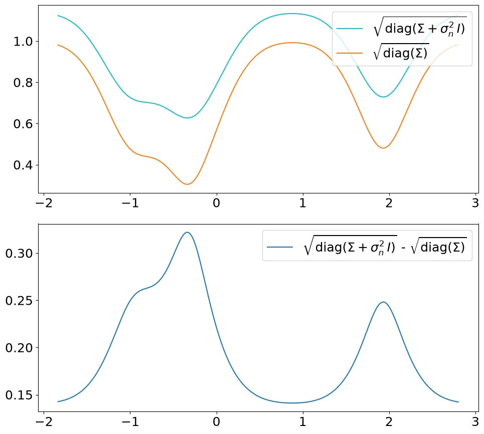
The only difference is that we now use the covariance matrix \(\ma\Sigma + \sigma_n^2\,\ma I\) instead of \(\ma\Sigma\) to generate samples from the posterior. By that we get (1) noisy samples and (2) a larger \(\sigma\). That’s what is typically not shown in text books (at least not the ones we checked). Noisy samples (only for the prior, but still) are shown for instance in [DLvdW20] in fig. 4.

The difference in \(\sigma\) between predict vs. predict_noiseless is not constant even though the constant \(\sigma_n^2\) is added to the diagonal because of the \(\sqrt{\cdot}\) in

\[\sigma = \sqrt{\mathrm{diag}(\cov(\ve f_*) + \sigma_n^2\ma I)}\]

../../_images/b7f3e28a4e0b70a5525d61f60f4e0b7502938e19c76b6132a9df6f5f7953e11a.png

../../_images/cff6bdabd500e583e47bb942de58d40800453f06b69171bf735fb1ff564bf99c.png