2D exact GP regression

In this notebook, we use a GP to fit a 2D data set. We use the same ExactGP machinery as in the 1D case and show how GPs can be used for 2D interpolation (when data is free of noise) or regression (noisy data). Think of this as a toy geospatial data setting. Actually, in geostatistics, Gaussian process regression is known as Kriging. \(\newcommand{\ve}[1]{\mathit{\boldsymbol{#1}}}\) \(\newcommand{\ma}[1]{\mathbf{#1}}\) \(\newcommand{\pred}[1]{\rm{#1}}\) \(\newcommand{\predve}[1]{\mathbf{#1}}\) \(\newcommand{\test}[1]{#1_*}\) \(\newcommand{\testtest}[1]{#1_{**}}\) \(\DeclareMathOperator{\diag}{diag}\) \(\DeclareMathOperator{\cov}{cov}\) \(\DeclareMathOperator{\sinc}{sinc}\)

##%matplotlib notebook
##%matplotlib widget
%matplotlib inline

from collections import defaultdict
from pprint import pprint

import torch
import gpytorch
from matplotlib import pyplot as plt
from matplotlib import is_interactive
import numpy as np

from sklearn.preprocessing import StandardScaler

from utils import extract_model_params, fig_ax_3d

torch.set_default_dtype(torch.float64)
torch.manual_seed(123)

<torch._C.Generator at 0x7fb280a23cb0>

Generate toy 2D data

Our ground truth function is \(f(\ve x) = \sin(r) / r\) (also known as \(\sinc(r)\)) with \(\ve x = [x_0,x_1] \in\mathbb R^2\) and the radial distance \(r=\sqrt{\ve x^\top\,\ve x}\). This creates a radial wave-like pattern which decays with distance from the center \(\ve x=\ve 0\). We generate data by random sampling 2D points \(\ve x_i\) and calculating \(y_i = f(\ve x_i)\), optionally adding Gaussian noise further down.

class Sinc:
    def __init__(self, xlim, ylim, nx, ny, mode, **kwds):
        self.xlim = xlim
        self.ylim = ylim
        self.nx = nx
        self.ny = ny
        self.xg, self.yg = self._get_xy_grid()
        self.XG, self.YG = self._get_meshgrids(self.xg, self.yg)
        self.X = self._make_X(mode)
        self.z = self.func(self.X)

    def _make_X(self, mode="grid"):
        if mode == "grid":
            X = torch.empty((self.nx * self.ny, 2))
            X[:, 0] = self.XG.flatten()
            X[:, 1] = self.YG.flatten()
        elif mode == "rand":
            X = torch.rand(self.nx * self.ny, 2)
            X[:, 0] = X[:, 0] * (self.xlim[1] - self.xlim[0]) + self.xlim[0]
            X[:, 1] = X[:, 1] * (self.ylim[1] - self.ylim[0]) + self.ylim[0]
        return X

    def _get_xy_grid(self):
        x = torch.linspace(self.xlim[0], self.xlim[1], self.nx)
        y = torch.linspace(self.ylim[0], self.ylim[1], self.ny)
        return x, y

    @staticmethod
    def _get_meshgrids(xg, yg):
        return torch.meshgrid(xg, yg, indexing="ij")

    @staticmethod
    def func(X):
        r = torch.sqrt((X**2).sum(axis=1))
        return torch.sin(r) / r

    @staticmethod
    def n2t(x):
        return torch.from_numpy(x)

    def apply_scalers(self, x_scaler, y_scaler):
        self.X = self.n2t(x_scaler.transform(self.X))
        Xtmp = x_scaler.transform(torch.stack((self.xg, self.yg), dim=1))
        self.XG, self.YG = self._get_meshgrids(
            self.n2t(Xtmp[:, 0]), self.n2t(Xtmp[:, 1])
        )
        self.z = self.n2t(y_scaler.transform(self.z[:, None])[:, 0])

Helper function for exercises

# Define GP model, same as in 1D notebook
class ExactGPModel(gpytorch.models.ExactGP):
    """API:

    model.forward()             prior                   f_pred
    model()                     posterior               f_pred

    likelihood(model.forward()) prior with noise        y_pred
    likelihood(model())         posterior with noise    y_pred
    """

    def __init__(self, X_train, y_train, likelihood):
        super().__init__(X_train, y_train, likelihood)
        self.mean_module = gpytorch.means.ConstantMean()
        self.covar_module = gpytorch.kernels.ScaleKernel(
            gpytorch.kernels.RBFKernel()
        )

    def forward(self, x):
        """The prior, defined in terms of the mean and covariance function."""
        mean_x = self.mean_module(x)
        covar_x = self.covar_module(x)
        return gpytorch.distributions.MultivariateNormal(mean_x, covar_x)

This function contains all the code of the 1D notebook plus some more plotting. It creates the 2D train data set, creates the GP model, runs the hyper parameter optimization and plots results. We will re-use this to cover different cases in the exercises below.

def run_example(use_noise: bool = False, use_gap: bool = False):
    """
    Parameters
    ----------
    use_noise
        Add Gaussian noise to training data
    use_gap
        Create a out-of-distribution region (a "gap") in the training data
    """

    data_train = Sinc(xlim=[-15, 25], ylim=[-15, 5], nx=20, ny=20, mode="rand")
    x_scaler = StandardScaler().fit(data_train.X)
    y_scaler = StandardScaler().fit(data_train.z[:, None])
    data_train.apply_scalers(x_scaler, y_scaler)

    data_pred = Sinc(
        xlim=[-15, 25], ylim=[-15, 5], nx=100, ny=100, mode="grid"
    )
    data_pred.apply_scalers(x_scaler, y_scaler)

    # train inputs
    X_train = data_train.X

    # inputs for prediction and plotting ("test data")
    X_pred = data_pred.X

    if use_noise:
        # noisy train data
        noise_std = 0.2
        noise_dist = torch.distributions.Normal(loc=0, scale=noise_std)
        y_train = data_train.z + noise_dist.sample(
            sample_shape=(len(data_train.z),)
        )
    else:
        # noise-free train data
        noise_std = 0
        y_train = data_train.z

    # Cut out part of the train data to create out-of-distribution predictions.
    # Same as the "gaps" we created in the 1D case.
    if use_gap:
        mask = (X_train[:, 0] > 0) & (X_train[:, 1] < 0)
        X_train = X_train[~mask, :]
        y_train = y_train[~mask]

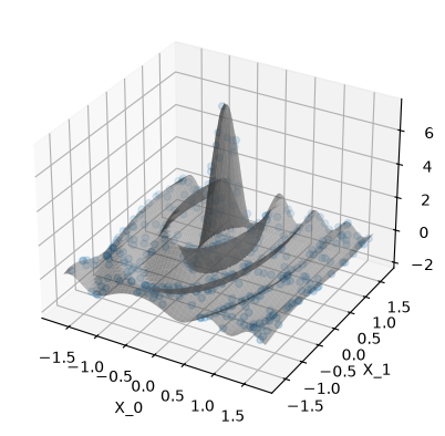
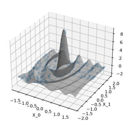
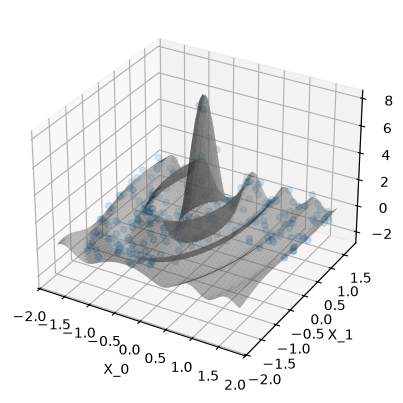
    print(
        "Plot the data. The gray surface is the ground truth function. "
        "The blue points are the training data."
    )

    fig, ax = fig_ax_3d()
    s0 = ax.plot_surface(
        data_pred.XG,
        data_pred.YG,
        data_pred.z.reshape((data_pred.nx, data_pred.ny)),
        color="tab:grey",
        alpha=0.5,
    )
    s1 = ax.scatter(
        xs=X_train[:, 0],
        ys=X_train[:, 1],
        zs=y_train,
        color="tab:blue",
        alpha=0.5,
    )
    ax.set_xlabel("X_0")
    ax.set_ylabel("X_1")

    if is_interactive():
        plt.show()

    likelihood = gpytorch.likelihoods.GaussianLikelihood()
    model = ExactGPModel(X_train, y_train, likelihood)

    print("\nInspect the model:")
    print(model)

    print("\nDefault start hyper params:")
    pprint(extract_model_params(model))

    # Set new start hyper params
    model.mean_module.constant = 0.0
    model.covar_module.base_kernel.lengthscale = 3.0
    model.covar_module.outputscale = 8.0
    model.likelihood.noise_covar.noise = 0.1

    pprint(extract_model_params(model))

    print("\nFit GP to data: optimize hyper params:")
    # Train mode
    model.train()
    likelihood.train()

    optimizer = torch.optim.Adam(model.parameters(), lr=0.15)
    loss_func = gpytorch.mlls.ExactMarginalLogLikelihood(likelihood, model)

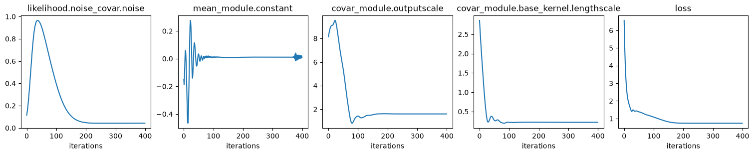
    n_iter = 400
    history = defaultdict(list)
    for ii in range(n_iter):
        optimizer.zero_grad()
        loss = -loss_func(model(X_train), y_train)
        loss.backward()
        optimizer.step()
        if (ii + 1) % 10 == 0:
            print(f"iter {ii + 1}/{n_iter}, {loss=:.3f}")
        for p_name, p_val in extract_model_params(
            model, try_item=True
        ).items():
            history[p_name].append(p_val)
        history["loss"].append(loss.item())

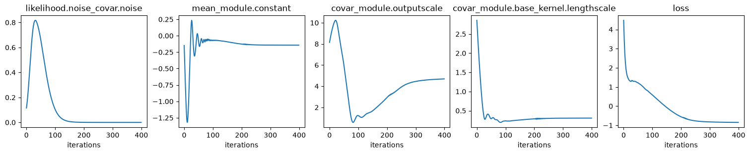
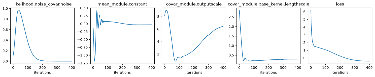
    ncols = len(history)
    fig, axs = plt.subplots(
        ncols=ncols, nrows=1, figsize=(ncols * 3, 3), layout="compressed"
    )
    with torch.no_grad():
        for ax, (p_name, p_lst) in zip(axs, history.items()):
            ax.plot(p_lst)
            ax.set_title(p_name)
            ax.set_xlabel("iterations")

    if is_interactive():
        plt.show()

    print("\nValues of optimized hyper params:")
    pprint(extract_model_params(model))

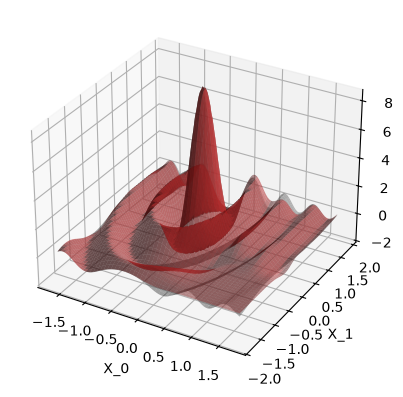
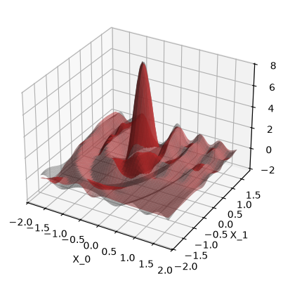
    print("\nPlot prediction:")
    model.eval()
    likelihood.eval()

    with torch.no_grad():
        post_pred_f = model(X_pred)
        post_pred_y = likelihood(model(X_pred))

        fig, ax = fig_ax_3d()
        ax.plot_surface(
            data_pred.XG,
            data_pred.YG,
            data_pred.z.reshape((data_pred.nx, data_pred.ny)),
            color="tab:grey",
            alpha=0.5,
        )
        ax.plot_surface(
            data_pred.XG,
            data_pred.YG,
            post_pred_y.mean.reshape((data_pred.nx, data_pred.ny)),
            color="tab:red",
            alpha=0.5,
        )
        ax.set_xlabel("X_0")
        ax.set_ylabel("X_1")

    assert (post_pred_f.mean == post_pred_y.mean).all()

    if is_interactive():
        plt.show()

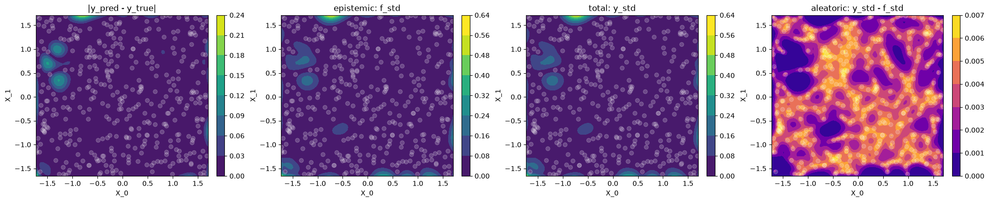
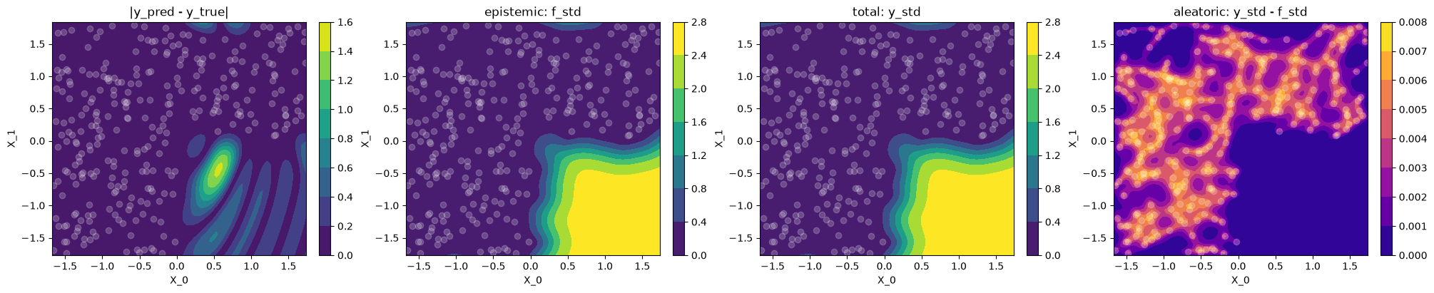
    print("""
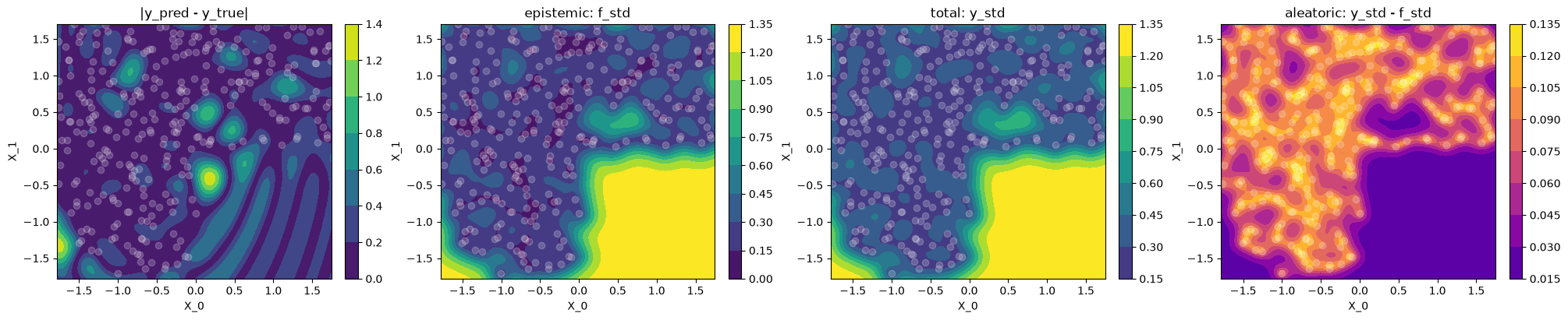
    Plot difference to ground truth and uncertainty

    Let's use contour plots to visualize the difference between GP prediction and
    ground truth, as well as epistemic, total and aleatoric uncertainty.
    """)

    ncols = 4
    fig, axs = plt.subplots(
        ncols=ncols, nrows=1, figsize=(ncols * 5, 4), layout="compressed"
    )

    vmax = post_pred_y.stddev.max()
    cs = []

    cs.append(
        axs[0].contourf(
            data_pred.XG,
            data_pred.YG,
            torch.abs(post_pred_y.mean - data_pred.z).reshape(
                (data_pred.nx, data_pred.ny)
            ),
        )
    )
    axs[0].set_title("|y_pred - y_true|")

    f_std = post_pred_f.stddev.reshape((data_pred.nx, data_pred.ny))
    y_std = post_pred_y.stddev.reshape((data_pred.nx, data_pred.ny))

    cs.append(
        axs[1].contourf(
            data_pred.XG,
            data_pred.YG,
            f_std,
            vmin=0,
            vmax=vmax,
        )
    )
    axs[1].set_title("epistemic: f_std")

    cs.append(
        axs[2].contourf(
            data_pred.XG,
            data_pred.YG,
            y_std,
            vmin=0,
            vmax=vmax,
        )
    )
    axs[2].set_title("total: y_std")

    cs.append(
        axs[3].contourf(
            data_pred.XG,
            data_pred.YG,
            y_std - f_std,
            vmin=0,
            cmap="plasma",
            ##vmax=vmax,
        )
    )
    axs[3].set_title("aleatoric: y_std - f_std")

    for ax, c in zip(axs, cs):
        ax.set_xlabel("X_0")
        ax.set_ylabel("X_1")
        ax.scatter(x=X_train[:, 0], y=X_train[:, 1], color="white", alpha=0.2)
        fig.colorbar(c, ax=ax)

    if is_interactive():
        plt.show()

    print("\nLet's check the learned noise:")

    # Target noise to learn
    print("data noise:", noise_std)

    # The two below must be the same
    print(
        "learned noise:",
        (post_pred_y.stddev**2 - post_pred_f.stddev**2).mean().sqrt().item(),
    )
    print(
        "learned noise:",
        np.sqrt(
            extract_model_params(model, try_item=True)[
                "likelihood.noise_covar.noise"
            ]
        ),
    )

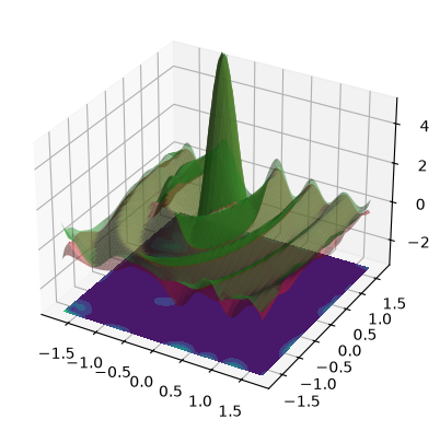
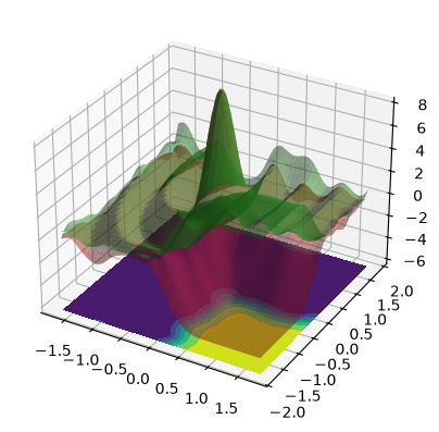
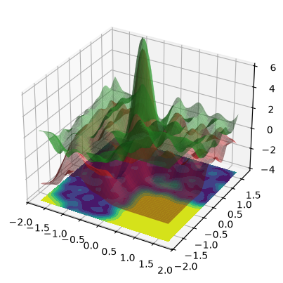
    print("\n3D confidence bands:")
    y_mean = post_pred_y.mean.reshape((data_pred.nx, data_pred.ny))
    y_std = post_pred_y.stddev.reshape((data_pred.nx, data_pred.ny))
    upper = y_mean + 2 * y_std
    lower = y_mean - 2 * y_std

    fig, ax = fig_ax_3d()
    for Z, color in [(upper, "tab:green"), (lower, "tab:red")]:
        ax.plot_surface(
            data_pred.XG,
            data_pred.YG,
            Z,
            color=color,
            alpha=0.5,
        )

    contour_z = lower.min() - 1
    zlim = ax.get_xlim()
    ax.set_zlim((contour_z, zlim[1] + abs(contour_z)))
    ax.contourf(data_pred.XG, data_pred.YG, y_std, zdir="z", offset=contour_z)

    if is_interactive():
        plt.show()

Run exercises

We have the following uncertainty terms:

• epistemic: f_std = \(\sqrt{\diag\test{\ma\Sigma}}\)

• total: y_std = \(\sqrt{\diag(\test{\ma\Sigma} + \sigma_n^2\,\ma I_N)}\)

• aleatoric: we have two ways of representing it

  • from the likelihood: \(\sigma_n\)

  • for plotting: we use y_std - f_std, this is \(\neq \sigma_n\) because of the \(\sqrt{\cdot}\) above

Exercise 1

run_example(use_noise=False, use_gap=False)

Plot the data. The gray surface is the ground truth function. The blue points are the training data.

Inspect the model:
ExactGPModel(
  (likelihood): GaussianLikelihood(
    (noise_covar): HomoskedasticNoise(
      (raw_noise_constraint): GreaterThan(1.000E-04)
    )
  )
  (mean_module): ConstantMean()
  (covar_module): ScaleKernel(
    (base_kernel): RBFKernel(
      (raw_lengthscale_constraint): Positive()
    )
    (raw_outputscale_constraint): Positive()
  )
)

Default start hyper params:
{'covar_module.base_kernel.lengthscale': tensor([[0.6931]], grad_fn=<SoftplusBackward0>),
 'covar_module.outputscale': tensor(0.6931, grad_fn=<SoftplusBackward0>),
 'likelihood.noise_covar.noise': tensor([0.6932], grad_fn=<AddBackward0>),
 'mean_module.constant': Parameter containing:
tensor(0., requires_grad=True)}
{'covar_module.base_kernel.lengthscale': tensor([[3.]], grad_fn=<SoftplusBackward0>),
 'covar_module.outputscale': tensor(8., grad_fn=<SoftplusBackward0>),
 'likelihood.noise_covar.noise': tensor([0.1000], grad_fn=<AddBackward0>),
 'mean_module.constant': Parameter containing:
tensor(0., requires_grad=True)}

Fit GP to data: optimize hyper params:
iter 10/400, loss=1.835
iter 20/400, loss=1.356
iter 30/400, loss=1.340
iter 40/400, loss=1.294
iter 50/400, loss=1.223
iter 60/400, loss=1.124
iter 70/400, loss=0.986
iter 80/400, loss=0.843
iter 90/400, loss=0.723
iter 100/400, loss=0.594
iter 110/400, loss=0.458
iter 120/400, loss=0.323
iter 130/400, loss=0.190
iter 140/400, loss=0.061
iter 150/400, loss=-0.062
iter 160/400, loss=-0.178
iter 170/400, loss=-0.286
iter 180/400, loss=-0.385
iter 190/400, loss=-0.475
iter 200/400, loss=-0.553
iter 210/400, loss=-0.606
iter 220/400, loss=-0.672
iter 230/400, loss=-0.710
iter 240/400, loss=-0.745
iter 250/400, loss=-0.770
iter 260/400, loss=-0.788
iter 270/400, loss=-0.801
iter 280/400, loss=-0.811
iter 290/400, loss=-0.819
iter 300/400, loss=-0.825
iter 310/400, loss=-0.830
iter 320/400, loss=-0.834
iter 330/400, loss=-0.837
iter 340/400, loss=-0.840
iter 350/400, loss=-0.842
iter 360/400, loss=-0.844
iter 370/400, loss=-0.846
iter 380/400, loss=-0.847
iter 390/400, loss=-0.849
iter 400/400, loss=-0.850

Values of optimized hyper params:
{'covar_module.base_kernel.lengthscale': tensor([[0.3063]], grad_fn=<SoftplusBackward0>),
 'covar_module.outputscale': tensor(4.6931, grad_fn=<SoftplusBackward0>),
 'likelihood.noise_covar.noise': tensor([0.0001], grad_fn=<AddBackward0>),
 'mean_module.constant': Parameter containing:
tensor(-0.1436, requires_grad=True)}

Plot prediction:

    Plot difference to ground truth and uncertainty

    Let's use contour plots to visualize the difference between GP prediction and
    ground truth, as well as epistemic, total and aleatoric uncertainty.

Let's check the learned noise:
data noise: 0
learned noise: 0.01054582313720995
learned noise: 0.01054582313720995

3D confidence bands:

When use_noise=False, then the GP’s prediction is an almost perfect reconstruction of the ground truth function (in-distribution, so where we have data). In this case, the plot makes the GP prediction look like a perfect interpolation of the noise-free data, so \(\test{\ve\mu} = \ve y\) at the train points \(\test{\ma X} = \ma X\). This would be true if our GP model had exactly zero noise, so the likelihood’s \(\sigma_n^2\) would be zero. However print(model)

ExactGPModel(
 (likelihood): GaussianLikelihood(
   (noise_covar): HomoskedasticNoise(
     (raw_noise_constraint): GreaterThan(1.000E-04)
   )
 )
 ...

shows that actually the min value is \(10^{-4}\), so we technically always have a regression setting, just with very small noise. The reason is that in the GP equations, the GP mean prediction at test points \(\test{\ma X}\) is given by

\[\test{\ve\mu} = \test{\ma K}\,\left(\ma K+\sigma_n^2\,\ma I_N\right)^{-1}\,\ve y\]

where \(\sigma_n^2\) acts as a regularization parameter (also called “jitter term” sometimes), which improves the numerical stability of the linear system solve step

\[\left(\ma K+\sigma_n^2\,\ma I_N\right)^{-1}\,\ve y\:.\]

Also we always keep \(\sigma_n^2\) as hyper parameter that we learn, and the smallest value the hyper parameter optimization can reach is \(10^{-4}\).

Observations

• use_noise=False, use_gap=False

  • The epistemic uncertainty f_std is a good indicator of the (small) differences between model prediction and ground truth (correlates with |y_pred - y_true|)

  • The learned variance \(\sigma_n^2\), and hence the aleatoric uncertainty is near zero, which makes sense for noise-free data, hence f_std and y_std are basically identical

  • The aleatoric y_std - f_std (4th plot) is not constant, and in particular \(\neq \sigma_n\) (learned noise) because we compare standard deviations and not variances.

Exercise 2

run_example(use_noise=False, use_gap=True)

Plot the data. The gray surface is the ground truth function. The blue points are the training data.

Inspect the model:
ExactGPModel(
  (likelihood): GaussianLikelihood(
    (noise_covar): HomoskedasticNoise(
      (raw_noise_constraint): GreaterThan(1.000E-04)
    )
  )
  (mean_module): ConstantMean()
  (covar_module): ScaleKernel(
    (base_kernel): RBFKernel(
      (raw_lengthscale_constraint): Positive()
    )
    (raw_outputscale_constraint): Positive()
  )
)

Default start hyper params:
{'covar_module.base_kernel.lengthscale': tensor([[0.6931]], grad_fn=<SoftplusBackward0>),
 'covar_module.outputscale': tensor(0.6931, grad_fn=<SoftplusBackward0>),
 'likelihood.noise_covar.noise': tensor([0.6932], grad_fn=<AddBackward0>),
 'mean_module.constant': Parameter containing:
tensor(0., requires_grad=True)}
{'covar_module.base_kernel.lengthscale': tensor([[3.]], grad_fn=<SoftplusBackward0>),
 'covar_module.outputscale': tensor(8., grad_fn=<SoftplusBackward0>),
 'likelihood.noise_covar.noise': tensor([0.1000], grad_fn=<AddBackward0>),
 'mean_module.constant': Parameter containing:
tensor(0., requires_grad=True)}

Fit GP to data: optimize hyper params:
iter 10/400, loss=2.428
iter 20/400, loss=1.676
iter 30/400, loss=1.469
iter 40/400, loss=1.427
iter 50/400, loss=1.373
iter 60/400, loss=1.307
iter 70/400, loss=1.243
iter 80/400, loss=1.196
iter 90/400, loss=1.137
iter 100/400, loss=1.072
iter 110/400, loss=1.000
iter 120/400, loss=0.922
iter 130/400, loss=0.839
iter 140/400, loss=0.753
iter 150/400, loss=0.665
iter 160/400, loss=0.577
iter 170/400, loss=0.491
iter 180/400, loss=0.406
iter 190/400, loss=0.325
iter 200/400, loss=0.246
iter 210/400, loss=0.172
iter 220/400, loss=0.101
iter 230/400, loss=0.034
iter 240/400, loss=-0.028
iter 250/400, loss=-0.086
iter 260/400, loss=-0.139
iter 270/400, loss=-0.186
iter 280/400, loss=-0.229
iter 290/400, loss=-0.253
iter 300/400, loss=-0.298
iter 310/400, loss=-0.325
iter 320/400, loss=-0.348
iter 330/400, loss=-0.366
iter 340/400, loss=-0.382
iter 350/400, loss=-0.394
iter 360/400, loss=-0.405
iter 370/400, loss=-0.413
iter 380/400, loss=-0.420
iter 390/400, loss=-0.426
iter 400/400, loss=-0.431

Values of optimized hyper params:
{'covar_module.base_kernel.lengthscale': tensor([[0.2960]], grad_fn=<SoftplusBackward0>),
 'covar_module.outputscale': tensor(6.4236, grad_fn=<SoftplusBackward0>),
 'likelihood.noise_covar.noise': tensor([0.0001], grad_fn=<AddBackward0>),
 'mean_module.constant': Parameter containing:
tensor(-0.0338, requires_grad=True)}

Plot prediction:

    Plot difference to ground truth and uncertainty

    Let's use contour plots to visualize the difference between GP prediction and
    ground truth, as well as epistemic, total and aleatoric uncertainty.

Let's check the learned noise:
data noise: 0
learned noise: 0.011906207140339081
learned noise: 0.01190620714033966

3D confidence bands:

Observations

• use_noise=False, use_gap=True

  • in-distribution (where we have data)

    • same as Exercise 1

  • out-of-distribution

    • When faced with out-of-distribution (OOD) data, the epistemic f_std clearly shows where the model will make wrong (less trustworthy) predictions

    • epistemic uncertainty f_std dominates and the aleatoric y_std - f_std vanishes

Exercise 3

run_example(use_noise=True, use_gap=True)

Plot the data. The gray surface is the ground truth function. The blue points are the training data.

Inspect the model:
ExactGPModel(
  (likelihood): GaussianLikelihood(
    (noise_covar): HomoskedasticNoise(
      (raw_noise_constraint): GreaterThan(1.000E-04)
    )
  )
  (mean_module): ConstantMean()
  (covar_module): ScaleKernel(
    (base_kernel): RBFKernel(
      (raw_lengthscale_constraint): Positive()
    )
    (raw_outputscale_constraint): Positive()
  )
)

Default start hyper params:
{'covar_module.base_kernel.lengthscale': tensor([[0.6931]], grad_fn=<SoftplusBackward0>),
 'covar_module.outputscale': tensor(0.6931, grad_fn=<SoftplusBackward0>),
 'likelihood.noise_covar.noise': tensor([0.6932], grad_fn=<AddBackward0>),
 'mean_module.constant': Parameter containing:
tensor(0., requires_grad=True)}
{'covar_module.base_kernel.lengthscale': tensor([[3.]], grad_fn=<SoftplusBackward0>),
 'covar_module.outputscale': tensor(8., grad_fn=<SoftplusBackward0>),
 'likelihood.noise_covar.noise': tensor([0.1000], grad_fn=<AddBackward0>),
 'mean_module.constant': Parameter containing:
tensor(0., requires_grad=True)}

Fit GP to data: optimize hyper params:
iter 10/400, loss=2.539
iter 20/400, loss=1.674
iter 30/400, loss=1.484
iter 40/400, loss=1.430
iter 50/400, loss=1.383
iter 60/400, loss=1.328
iter 70/400, loss=1.255
iter 80/400, loss=1.199
iter 90/400, loss=1.144
iter 100/400, loss=1.089
iter 110/400, loss=1.030
iter 120/400, loss=0.970
iter 130/400, loss=0.913
iter 140/400, loss=0.861
iter 150/400, loss=0.818
iter 160/400, loss=0.785
iter 170/400, loss=0.762
iter 180/400, loss=0.748
iter 190/400, loss=0.742
iter 200/400, loss=0.739
iter 210/400, loss=0.738
iter 220/400, loss=0.738
iter 230/400, loss=0.738
iter 240/400, loss=0.738
iter 250/400, loss=0.738
iter 260/400, loss=0.738
iter 270/400, loss=0.738
iter 280/400, loss=0.738
iter 290/400, loss=0.738
iter 300/400, loss=0.738
iter 310/400, loss=0.738
iter 320/400, loss=0.738
iter 330/400, loss=0.738
iter 340/400, loss=0.738
iter 350/400, loss=0.738
iter 360/400, loss=0.738
iter 370/400, loss=0.738
iter 380/400, loss=0.738
iter 390/400, loss=0.738
iter 400/400, loss=0.738

Values of optimized hyper params:
{'covar_module.base_kernel.lengthscale': tensor([[0.2231]], grad_fn=<SoftplusBackward0>),
 'covar_module.outputscale': tensor(1.6015, grad_fn=<SoftplusBackward0>),
 'likelihood.noise_covar.noise': tensor([0.0428], grad_fn=<AddBackward0>),
 'mean_module.constant': Parameter containing:
tensor(0.0085, requires_grad=True)}

Plot prediction:

    Plot difference to ground truth and uncertainty

    Let's use contour plots to visualize the difference between GP prediction and
    ground truth, as well as epistemic, total and aleatoric uncertainty.

Let's check the learned noise:
data noise: 0.2
learned noise: 0.20693478466819767
learned noise: 0.20693478466819765

3D confidence bands:

Observations

• use_noise=True, use_gap=True

  • in-distribution (where we have data)

    • The epistemic (f_std) uncertainty’s interpretation is less clear since f_std doesn’t correlate well with y_pred - y_true as it did in the noise-free case. The reason is that the noise \(\sigma_n\) shows up in two parts: (a) in the equation of \(\test{\ma\Sigma}\) itself, so the “epistemic” uncertainty f_std = \(\sqrt{\diag\test{\ma\Sigma}}\) is bigger just because we have noise (regression) and (b) we add it in \(\sqrt{\diag(\test{\ma\Sigma} + \sigma_n^2\,\ma I_N)}\) to get the total y_std

  • out-of-distribution

    • same as Exercise 2

# When running as script
if not is_interactive():
    plt.show()