Velocity autocorrelation function and phonon DOS
Correlation and power spectrum
Here are some (textbook) notes about correlation, which you should read in
order to understand how the phonon DOS (= vibrational density of states =
power spectrum of the atomic velocities) is calculated in pwtools (see
pydos).
The cross-correlation theorem for the two-sided correlation:
corr(a,b) = ifft(fft(a)*fft(b).conj())
If a == b, then this reduces to the special case of the Wiener-Khinchin theorem (autocorrelation of a):
corr(a,a) = ifft(abs(fft(a))**2)
where the power spectrum of a is simply:
fft(corr(a,a)) == abs(fft(a))**2
Both theorems assume periodic data, i.e. a and b repeat after nstep
points. To deal with non-periodic data, we use zero-padding with nstep-1
points at the end of a before fft. Therefore, the correlated signal is
2*nstep-1 points long (“two-sided correlation”) and contains the correlations for positive and
negative lags. Since the autocorrelation function is symmetric around lag=0, we
return 0 … +lag in pwtools.signal.acorr(). To compare that with
scipy.signal.correlate(a,a,'full'), we need to mirror the result at lag=0
again.
Here are these equalities with discrete data. Note that due to the
way in which fft/ifft packs the data in the returned array, we need
to do some slicing + mirror tricks to get it right. In each example,
the arrays c1,c2,c3 and p1,p2 are the same and for corr(v,v) we use
acorr(v) here.
Two-sided correlation for -lag…0…+lag:
>>> from pwtools.signal import pad_zeros, welch, mirror, acorr
>>> from scipy.signal import correlate
>>> from scipy.fftpack import fft,ifft
>>> pad=lambda x: pad_zeros(x, nadd=len(x)-1)
>>> n=500; w=welch(n)
>>> t=linspace(0,1,n); dt=t[1]-t[0]
>>> v=np.array([sin(2*pi*f*t + rand()*2*pi) for f in rand(10)*100]).sum(0)
>>> f=np.fft.fftfreq(2*n-1, dt)[:n]
>>> figure(); plot(t,v); title('signal')

>>> c1=mirror(ifft(abs(fft(pad(v)))**2.0)[:n].real)
>>> c2=correlate(v,v,'full')
>>> c3=mirror(acorr(v,norm=False))
>>> figure(); plot(c1, label='fft'); plot(c2, label='scipy'); \
... plot(c3, label='acorr'); title('corr'); legend()
and the power spectra as fft(corr(v,v)), now one-sided:
>>> p1=(abs(fft(pad(v)))**2.0)[:n]
>>> p2=(abs(fft(mirror(acorr(v,norm=False)))))[:n]
>>> figure(); plot(f,p1, label='fft'); plot(f,p2, label='acorr'); \
... title('spectrum'); legend()
also with a Welch window:
>>> p1=(abs(fft(pad(v*w)))**2.0)[:n]
>>> p2=(abs(fft(mirror(acorr(v*w,norm=False)))))[:n]
>>> figure(); plot(f,p1, label='fft'); plot(f,p2, label='acorr'); \
... title('spectrum welch'); legend()
The zero-padding before fft is manadatory! It is also done inside
scipy.signal.correlate().
The 1D reference implementation is pwtools.signal.acorr(), which contains the
fft-based correlation (Wiener-Khinchin) along with other methods.
Padding and smoothing
There is another code out there (appart from fourier.x from CPMD)
which calculates the phonon DOS from MD data. What they do is padding the
correlation function, i.e. something like fft(pad(acorr(v))), which is
not the same as fft(mirror(acorr(v))). They also use smoothing (convolution
with a gaussian, i.e. fft(smooth(pad(acorr(v))))) after padding, which is
less effective than using a Welch (or any other) window function. But we
haven’t tested the code, so all this may work just fine.
For smoothing the spectrum (e.g. p1=(abs(fft(pad(v)))**2.0)[:n]) using our
implementation, use pwtools.signal.smooth(), i.e. smooth(p1). For
increasing the interpolation, use more padding of the time series, for
instance pad_zeros(v, nadd=(len(v)-1)*5) instead of len(v)-1.
Calculation of the phonon DOS from MD data
The pydos module containes many helper and reference
implementations, but the the main function to be used is
pdos().
There are two ways of computing the phonon density of states (PDOS) from an MD
trajectory. v is the 3d array of atomic velocities with shape (nstep,natoms,3),
i.e. Trajectory.velocity, see velocity_traj().
method='vacf':fftof the velocity autocorrelation function (vacf):v->vacf->fft(vacf)= PDOS, seevacf_pdos()
method='direct':abs(fft(v))**2= PDOS, seedirect_pdos(),This is much faster and mathematically exactly the same, see
examples/examples/phonon_dosandtest/test_pdos.py.
Both methods are implemented but actually only method ‘direct’ is worth using. Method ‘vacf’ still exists for historical reasons and as reference.
The actual implementation is in pdos() and the above two
functions are convenience wrappers.
In method ‘vacf’, if we mirror the
vacfat t=0 before thefft, then we get double frequency resolution.By default,
direct_pdos()uses zero-padding ofvto get the same frequency resolution as we would get with mirroring the signal (mirr=True)vacf_pdos(). Also, padding is necessary b/c of the arguments outlined above for the 1d case.Both methods use Welch windowing by default to reduce “leakage” from neighboring peaks.
Both methods must produce exactly the same results (up to numerical noise).
The frequency axis of the PDOS is in Hz. It is “f”, NOT the angular frequency 2*pi*f. See also
examples/pdos_methods.py.- The difference to the 1d case:
mass weighting: this affects only the relative peak heights in the PDOS, not the peak positions
averaging over natoms to get a 1d array (time series)
