Radial Basis Function interpolation an regression
Note
While the material here is a useful reference and the code has been used in
production, we actually recommend to use Gaussian process regression
instead, e.g. sklearn.gaussian_process.GaussianProcessRegressor,
or, if you want to replicate rbf, then use KRR
(sklearn.kernel_ridge.KernelRidge). See
https://github.com/elcorto/gp_playground for a detailed comparison of GPs
and KRR.
Some background information on the method implemented in rbf.
For code examples, see the doc string of Rbf and
examples/rbf.
Theory
The goal is to interpolate or fit an unordered set of \(M\) ND data points \(\mathbf x_i\) and values \(z_i\) so as to obtain \(z=f(\mathbf x)\). In radial basis function (RBF) interpolation, the interpolating function \(f(\mathbf x)\) is a linear combination of RBFs \(\phi(r)\)
with the weights \(w_j\) and the center points \(\mathbf c_j\).
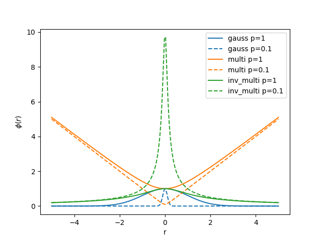
An RBF \(\phi(r)\) is a function of the distance \(r=|\mathbf x - \mathbf c_j|\) between \(\mathbf x\) and a center point. Common functions include
All RBFs contain a single parameter \(p\) which defines the length scale of the function.
In interpolation the center points \(\mathbf c_j\) are equal to the data points \(\mathbf x_j\) such that
with \(\mathbf K\) the \(M\times M\) matrix of RBF function values. The weights \(\mathbf w = (w_j)\) are found by solving the linear system \(\mathbf K\,\mathbf w = \mathbf z\).
Note that for certain values of \(p\), \(\mathbf K\) may become singular, esp. large ones with the limit being \(p\rightarrow\infty\Rightarrow\phi\rightarrow\text{const}\). Then one should solve a regression problem instead (see below).
RBF parameter \(p\)
Each RBF has a single “length scale” parameter \(p\) (Rbf(p=...),
attribute Rbf.p). While \(f(\mathbf x)\) goes through all points
(\(\mathbf x_i\), \(z_i\)) by definition in interpolation, the behavior
between points is determined by \(p\) where e.g. very narrow functions
\(\phi\) can lead to oscillations between points. Therefore \(p\) must
be optimized for the data set at hand, which should be done by cross-validation
as will be explained below.
Nevertheless we provide two methods to estimate reasonable start values.
The scipy implementation \(p_{\text{scipy}}\) in
scipy.interpolate.Rbf uses something like the mean nearest neighbor
distance. We provide this as Rbf(points, values, p='scipy') or
rbf.estimate_p(points, 'scipy'). The default in pwtools.rbf.Rbf
however is the mean distance of all points
Use Rbf(points, values, p='mean') or rbf.estimate_p(points, 'mean').
This is always bigger than \(p_{\text{scipy}}\) and can be a better start
guess for \(p\), especially in case of regression.
Interpolation vs. regression, regularization and numerical stability
In case of noisy data, we may want to do regression. Similar to the s
parameter of scipy.interpolate.bisplrep() or the smooth parameter for
regularization in scipy.interpolate.Rbf, we solve a regularized
version of the linear system
using, for instance, Rbf(points, values, r=1e-8) (attribute Rbf.r). The
default however is \(r=0\) (interpolation). \(r>0\) creates a more
“stiff” (low curvature) function \(f(\mathbf x)\) which does not
interpolate all points and where r is a measure of the assumed noise. If
the RBF happens to imply a Mercer kernel (which the Gaussian one does), then
this is equal to kernel ridge regression (KRR).
Apart from smoothing, the regularization also deals with the numerical instability of \(\mathbf K\,\mathbf w = \mathbf z\).
One can also switch from scipy.linalg.solve() to
scipy.linalg.lstsq() and solve the system in a least squares sense
without regularization. You can do that by setting Rbf(..., r=None). In
sklearn.kernel_ridge.KernelRidge there is an automatic switch to least
squares when a singular \(\mathbf K\) is detected. However, we observed
that in many cases this results in numerical noise in the solution, esp. when
\(\mathbf K\) is (near) singular. So while we provide that feature for
experimentation, we actually recommend not using it in production and instead
use a KRR setup and properly determine \(p\) and \(r\) as described
below.
How to determine \(p\) and \(r\)
\(p\) (and \(r\)) should always be tuned to the data set at hand by
minimization of a cross validation (CV) score. You can do this with
pwtools.rbf.hyperopt.fit_opt(). Here is an example where we optimize only
\(p\), with \(r\) constant and very small such as 1e-11. See
examples/rbf/overfit.py.
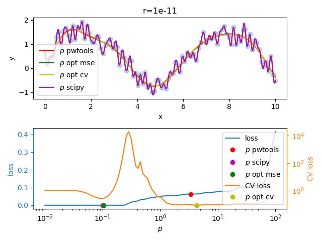
We observe a flat CV score above \(p>1\) without a pronounced global minimimum, even though we find a shallow one at around \(p=13\), while the MSE loss (fit error) would suggest a very small \(p\) value (i.e. interpolation or “zero training loss” in ML terms).
Now we investigate \(p\) and \(r\) (see
examples/rbf/crossval_map_p_r.py) by plotting the CV score as function of
both. This is the result for the Gaussian RBF.
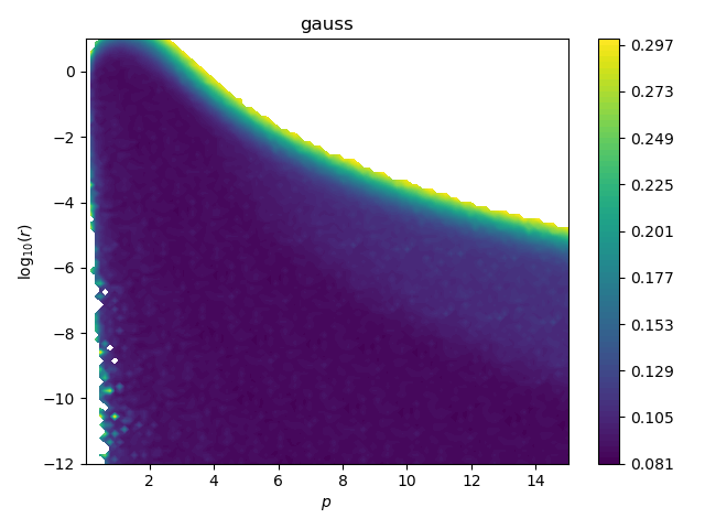
When \(r < 10^{-6}\), it basically doesn’t matter which \(p\) we use, as long as it is big enough to not overfit, i.e. \(p>1\). In these regions, both \(p\) and \(r\) provide stiffness. The large \(p\)-\(r\) valley of low CV score is flat and a bit rugged such that there is no pronounced global optimum, as shown above for \(r=10^{-11}\). As we incease \(r\) (stronger regularization = stronger smoothing) we are restricted to lower \(p\) (narrow RBFs which can overfit) since the now higher \(r\) already provides enough stiffness to prevent overfitting.
Data scaling
In pwtools.num.PolyFit (see the scale keyword) we scale
\(\mathbf x\) and \(z\) to \([0,1]\). Here we don’t have that
implemented but suggest to always scale at least \(z\). Since in contrast
to polynomials, the model here has no constant bias term, one should instead
normalize to zero mean using something like
sklearn.preprocessing.StandardScaler.