Tutorial
Here we collect random short code snippets showing how to perform various common tasks.
Using ASE?
No problem, use atoms2struct() and
struct2atoms() to convert back and forth. If you have a
Structure, you can also use the
get_ase_atoms() method, which is the same as
struct2atoms(struct).
For basic ASE compatibility, you may get away with
get_fake_ase_atoms(). That creates an object
which behaves like ase.Atoms without the need to have ASE installed.
Parse SCF, relax or MD output
Parse SCF run from QE (single Structure):
>>> from pwtools import io
>>> st = io.read_pw_scf('pw.scf.out')
>>> # natoms=2
>>> st.coords_frac
array([[0.  , 0.  , 0.  ],
       [0.25, 0.25, 0.25]])
>>> st.etot
-258.58148870118305
>>> st.stress
array([[9.825, 0.   , 0.   ],
       [0.   , 9.825, 0.   ],
       [0.   , 0.   , 9.825]])
Variable cell relax run from QE into Trajectory. Use the
MD parser:
>>> tr = io.read_pw_md('pw.vc_relax.out')
>>> tr.nstep
7
>>> tr.etot - tr.etot[-1]
array([-0.74763576,  0.68611164,  0.22244653, -0.06793023, -0.01616479,
        0.00121567,  0.        ])
>>> tr.volume
array([54.12697068, 51.59033133, 49.81153398, 50.1512203 , 50.26524368,
       50.25804864, 50.25804864])
>>> # [trace(s)/3 for s in tr.stress]
>>> tr.pressure
array([ 2.60203333e+01, -5.28800000e+00, -2.22400000e+00,  6.80000000e-01,
        1.14000000e-01, -6.30000000e-02, -2.33333333e-02])
>>> tr.cryst_const[-1,...]
array([  3.29944506,   3.29944506,   5.33081055,  90.        ,
        90.        , 120.00001397])
>>> # nstep=7, natoms=4
>>> tr.coords.shape
(7, 4, 3)
Now an MD from CP2K:
>>> tr = io.read_cp2k_md('cp2k.out')
>>> tr.nstep
123456
>>> # extract first and last Structure objects
>>> st_first = tr[0]
>>> st_last = tr[-1]
>>> # slice out a part of the trajectory
>>> tr_middle = tr[100:500]
>>> # use every 5th step
>>> tr[::5]
Binary IO
You can save a Structure or
Trajectory object as binary file:
>>> # save to binary pickle file
>>> tr.dump('traj.pk')
and read it back in later using read_pickle()
>>> tr = io.read_pickle('traj.pk')
which is usually very fast.
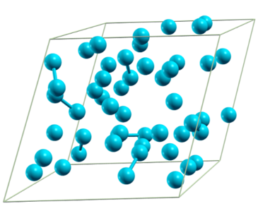
View a structure or trajectory
Supported viewers are xcrysden, jmol, avogadro and VMD. Look at single structs or trajectories.
>>> from pwtools import visualize, random
>>> st = random.random_struct(['Si']*50)
>>> visualize.view_xcrysden(st)
>>> ##visualize.view_jmol(st)
>>> ##visualize.view_avogadro(st)
Andf you have VMD installed, view a random MD trajectory:
>>> import os
>>> from pwtools import crys
>>> tr = crys.concatenate([random.random_struct(['Si']*10) for i in \
...                        range(5)])
>>> # vmd startup script
>>> vmd_script = os.path.dirname(visualize.__file__) + \
                                 '/examples/vmd/nice_bonds.tcl'

>>> visualize.view_vmd_axsf(tr, options='-e %s' %vmd_script)
Find Monkhorst-Pack k-grid sampling for a given unit cell
Say you know from a previous convergence study that a k-grid spacing of
h=0.5 1/Angstrom is OK. Now you have a slab or other super cell of your
structure and you want to know “what k-grid do I need to get the same
accuracy”. Simple:
>>> from pwtools import crys
>>> # new cell in Angstrom
>>> cell=np.diag([8,8,5])
>>> crys.kgrid(cell, h=0.5)
array([2, 2, 3])
OK, so use a \(2\times2\times3\) MP grid. Instead of defining cell by
hand, you could also build your structure, have it in a Structure object, say
st and use st.cell instead.
Find spacegroup
Say you have a Trajectory tr, which is the result of a relax calculation and you
want to know the space group of the final optimized structure, namely
tr[-1]:
>>> from pwtools import symmetry, crys
>>> symmetry.get_spglib_spacegroup(tr[-1], symprec=1e-2)
Or build one using ASE:
>>> import ase.build
>>> at = ase.build.bulk(name='AlN', crystalstructure='rocksalt', a=3)
>>> symmetry.spglib_get_spacegroup(crys.atoms2struct(at))
(225, 'Fm-3m')
Smoothing a signal or a Trajectory
Smoothing a signal (usually called “time series”) can be done by convolution
with another function (e.g. with scipy.signal.convolve or
scipy.signal.fftconvolve). We implement advanced methods which add edge
effect handling: pwtools.signal.smooth(). The same can be applied to a
Trajectory, which is just a “time series” of Structures. See
pwtools.crys.smooth():
>>> a = rand(10000)
>>> a_smooth = signal.smooth(a, scipy.signal.hann(151))
>>> tr = Trajectory(...)
>>> tr_smooth = crys.smooth(tr, scipy.signal.hann(151))
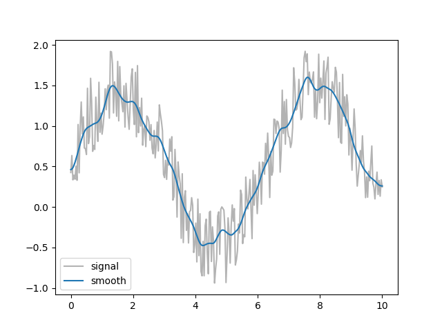
Example:
>>> from pwtools.signal import smooth
>>> from pwtools import mpl
>>> from scipy.signal import hann
>>> fig,ax = mpl.fig_ax()
>>> x = np.linspace(0,10,300)
>>> y = np.sin(x) + np.random.rand(len(x))
>>> k = hann(21)
>>> ax.plot(x, y, color='0.7', label='signal')
>>> ax.plot(x, smooth(y, k), label='smooth')
>>> ax.legend()
>>> mpl.plt.show()
The same is applied to each atomic coordinate in pwtools.crys.smooth().
Find more about edge effects in examples/lorentz.py and the doc string of
pwtools.signal.smooth().
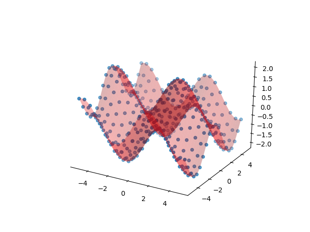
Interpolation and fitting
Care for some surface data? Here we fit with a 2D polynomial:
>>> from pwtools import num, rbf, mpl
>>> fig,ax = mpl.fig_ax3d(clean=True)
>>> dd = mpl.get_2d_testdata(20)
>>> ax.scatter(dd.xx, dd.yy, dd.zz)
>>> # same as
>>> #   num.Interpol2D(dd=dd, what='poly', deg=5)
>>> #   num.Interpol2D(dd.XY, dd.zz, what='poly', deg=5)
>>> f = num.PolyFit(dd.XY, dd.zz, deg=5)
>>> ddi = mpl.get_2d_testdata(50)
>>> ddi.update(zz=f(ddi.XY))
>>> ax.plot_surface(ddi.X, ddi.Y, ddi.Z, alpha=0.3, color='r')
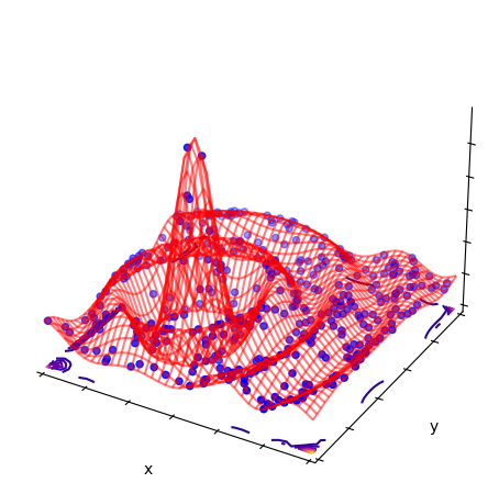
2D interpolation of samples of a “mexican hat” function \(\sin(r)/r\)
(examples/rbf/surface.py), also using Rbf. See
Radial Basis Function interpolation an regression for more. Similar to the PolyFit example above:
>>> # same as
>>> #   num.Interpol2D(dd=dd, what='rbf_multi')
>>> #   num.Interpol2D(dd.XY, dd.zz, what='rbf_multi')
>>> f=rbf.Rbf(dd.XY, dd.zz)
See also
Avoid auto-calculation for big MD data
If you have really big MD data (say several GB), then the auto-calculation of
missing properties might take long and/or fill
up all memory. To avoid that, call the parser explicitly and say
auto_calc=False when creating the Trajectory,
which will deactivate auto-calculation. It will only do unit conversion to eV,
Ang, etc. [you can of course also access the parser’s attributes directly, e.g.
pp.coords in the unit of the MD code (e.g. Bohr) instead of tr.coords
in Ang].
This is an example for parsing LAMMPS dcd binary data (log.lammps is the
logfile and the default binary file is lmp.out.dcd).
>>> pp = parse.LammpsDcdMDOutputFile('log.lammps')
>>> tr = pp.get_traj(auto_calc=False) # default is auto_calc=True
In order to maximally reduce data, you can tell the parser to parse only certain things:
>>> pp.set_attr_lst(['etot', 'coords', 'temperature'])
>>> tr = pp.get_traj(auto_calc=False)
You may also use auto_calc=True here and see what will be
auto-calculated from this minimal input data.
Of course you need to know what can be found in the MD data (e.g. if the MD
code writes no fractional coords, then parsing coords_frac won’t work).
To find out what can be parsed, also check which get_*() methods the parser
implements (mind also base classes, best is to use Tab completion in ipython:
>>> pp.get_<tab> or have a look at the API documentation).
Work with SQLite databases
See SQLiteDB.